
Published | Last updated
Competing risks are the reason a survival curve in an older cancer cohort can be confidently, reproducibly wrong. When a seventy-eight-year-old with a slow-growing tumour dies of heart failure, that death does not censor the cancer outcome. That death removes the possibility of the cancer outcome forever. Kaplan-Meier cannot represent that, because censoring in Kaplan-Meier means “we stopped watching”, not “this can no longer happen”. Apply it to cancer-specific death anyway and the estimate drifts upward in a direction you can predict but most published papers do not correct.
We wanted the size of the error rather than the principle, so we simulated it. Kaplan-Meier can overstate the ten-year cumulative incidence of cancer death by up to 19 percentage points. The result that surprised us is what happens next, when authors apply the fix reviewers ask for. Across 8,000 simulated studies, Fine-Gray reported a statistically significant effect in as many as 100 percent of them for a group difference that had precisely zero effect on the cancer.
In Simple Words
Imagine following a thousand elderly patients to see how many eventually die of their cancer. Some of them will die of a heart attack first. The usual survival method quietly assumes those people would have gone on to die of the cancer at the same rate as everyone else, which is not true, because they are already gone. So it reports a higher cancer death rate than the one the patients actually experienced. A correct method counts them properly. The complication is that there are two correct methods, they answer two different questions, and a paper that swaps one for the other can report a strong finding about a group whose cancer behaved identically.
What Competing Risks Actually Are
A competing risk is an event whose occurrence prevents the event you care about. In an oncology cohort followed for cancer-specific death, every other cause of death competes. Andersen and colleagues set out the framework in epidemiological terms, noting that the choice between analysing rates and analysing risks is a substantive question rather than a technical one (International Journal of Epidemiology 2012;41(3):861-870, doi:10.1093/ije/dyr213).
Two quantities matter and they are not the same thing. The cause-specific hazard is the instantaneous rate of cancer death among patients still alive and still at risk, which is the closest available proxy for how aggressively the tumour is behaving. The cumulative incidence function is the probability that a patient has died of cancer by a given time, in a real world where other causes of death are also operating, which is what a patient or a health system actually experiences.
Kaplan-Meier applied to cancer-specific death estimates neither. Austin, Lee and Fine stated the rule directly, that analysts estimating the crude incidence of outcomes should use the cumulative incidence function rather than the complement of the Kaplan-Meier survival function, because the Kaplan-Meier approach overestimates the event probability (Circulation 2016;133(6):601-609, doi:10.1161/CIRCULATIONAHA.115.017719). Our question was how much.
How Far Kaplan-Meier Overstates Cancer Death
We built cohorts with constant cause-specific hazards, one for cancer death and one for death from every other cause, followed for ten years. Under those conditions the true cumulative incidence of cancer death has a closed form, so the simulation has an exact answer to be checked against rather than a consensus to be negotiated.
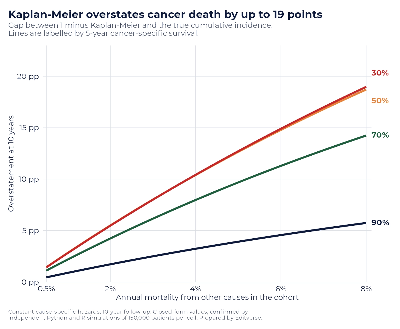
Where competing mortality is negligible, so is the error. A cohort with 90 percent five-year cancer-specific survival and only 0.5 percent annual other-cause mortality, roughly a young and otherwise healthy population, sees Kaplan-Meier report 19.00 percent against a true 18.55 percent at ten years. Less than half a percentage point, and no reviewer would notice.
Raise the competing mortality to 8 percent a year, which is an ordinary figure for a cohort in its eighties, and the picture changes completely. For a cancer with 70 percent five-year cancer-specific survival, Kaplan-Meier reports 51.00 percent while the truth is 36.76 percent. That is an absolute overstatement of 14.2 percentage points and a relative overstatement of 39 percent. Push the aggressiveness to 30 percent five-year survival and the absolute gap reaches 19.0 points, 91.00 percent against a true 72.03 percent.
| 5-year cancer-specific survival | Annual other-cause mortality | True cumulative incidence at 10 y | 1 minus Kaplan-Meier | Overstatement |
|---|---|---|---|---|
| 90% | 0.5% | 18.55% | 19.00% | +0.45 pp (2%) |
| 90% | 8% | 13.26% | 19.00% | +5.74 pp (43%) |
| 70% | 2% | 46.77% | 51.00% | +4.23 pp (9%) |
| 70% | 8% | 36.76% | 51.00% | +14.24 pp (39%) |
| 50% | 8% | 56.29% | 75.00% | +18.71 pp (33%) |
| 30% | 8% | 72.03% | 91.00% | +18.97 pp (26%) |
Two patterns are worth carrying into your own study. In absolute terms the damage is worst for aggressive cancers, because there is more probability mass available to misallocate. In relative terms it is worst for indolent ones, where a 5.7-point error on a true 13.3 percent is a 43 percent overstatement of the thing the paper is about. Neither reading is the safe one, and which matters depends on whether your conclusion is phrased as a percentage or as a ratio.
How We Tested This
Every figure above was produced twice, by two engines that share no code, no formulae and no random number stream. The Python engine draws exponential event times with NumPy and estimates the cumulative incidence with a hand-written Aalen-Johansen estimator. Running on a separate server, the R engine uses its own generator and the survival package, with the Aalen-Johansen step cross-checked against the package’s own multi-state estimator on a small cohort, where the two agreed to fourteen decimal places.
Both engines were then checked against the closed form. Across all twenty combinations of cancer aggressiveness and competing mortality, the largest discrepancy between simulation and closed form was 0.0017 for the cumulative incidence and 0.0024 for Kaplan-Meier, on cohorts of 150,000 patients per cell. That is Monte Carlo noise, which is the answer we wanted. A dual-engine gate is not there to make a result look thorough. Its purpose is narrower, because a single implementation of a survival estimator is a single point of failure, and a silent indexing error in a risk set produces numbers that look entirely plausible.
Fine-Gray Answers a Different Question
A reviewer who spots Kaplan-Meier on cancer-specific death will usually ask for Fine-Gray, the subdistribution hazard model that has become the standard regression tool for competing risks (Journal of the American Statistical Association 1999;94(446):496-509, doi:10.1080/01621459.1999.10474144). Authors comply, the model runs, the hazard ratio is reported, and the paper is accepted. We wanted to know what that hazard ratio means when the groups being compared differ in something other than their cancer.
So we built the cleanest possible test. Two groups, 2,000 patients, ten years of follow-up, and a cancer-specific hazard that is exactly identical in both groups. The only difference between them is mortality from other causes, set at 0.5 percent a year in one group and at 2, 5 or 10 percent in the other. Whatever the exposure is, it has no effect on the tumour. We fitted both a cause-specific Cox model and a Fine-Gray model to each simulated study, 2,000 studies per scenario in Python and 350 in R, and recorded how often each model would have been written up as a positive finding.

Identical cancer biology, a significant Fine-Gray result
The cause-specific Cox model behaved exactly as it should. Its median hazard ratio was 1.000 in Python and between 0.993 and 1.006 in R across the three scenarios, and it reached statistical significance in roughly 5 percent of studies, which is the nominal false positive rate and nothing more.
Fine-Gray did something else. At the mildest contrast, 0.5 percent against 2 percent annual competing mortality, the median subdistribution hazard ratio was 0.918 and about a third of studies reached significance, 31.7 percent in Python and 34.6 percent in R. At 0.5 against 5 percent the median fell to 0.79 and 97.8 percent of studies were significant. At 0.5 against 10 percent the median was 0.63 and every single one of the 2,000 simulated studies returned a statistically significant result, in both engines.
Read that as a published sentence and the problem is obvious. A paper would report a subdistribution hazard ratio of 0.63 with a confidence interval nowhere near unity, and a discussion section would explain why the exposure protects against cancer death. That exposure does nothing of the kind. By construction, the cancer-specific hazard is identical. What the model has detected, correctly, is that patients in the high-competing-mortality group are less likely to reach a cancer death because something else reaches them first.
The control condition
We ran a fourth scenario to confirm that the divergence comes from competing mortality rather than from anything else in the setup. Here the two groups had equal other-cause mortality at 2 percent a year and a genuine difference in the cancer, with five-year cancer-specific survival of 60 percent against 75 percent. Both models agreed closely, a cause-specific hazard ratio of 0.564 and a subdistribution hazard ratio of 0.573 in Python, with R returning 0.562 and 0.573. When the exposure acts on the tumour and nothing else, the two answers converge, which is exactly why their disagreement elsewhere is informative rather than a nuisance.
What each model actually estimates
Neither model is broken and neither is the safe default. Austin and Fine set out the distinction in the paper that has become the standard citation for this choice, explaining that the cause-specific hazard model addresses which covariates affect the rate at which events occur while the subdistribution hazard model addresses which covariates affect the probability of an event occurring over time (Statistics in Medicine 2017;36(27):4391-4400, doi:10.1002/sim.7501).
Translated into a cancer cohort, the cause-specific hazard ratio is the aetiological quantity. That quantity answers whether the exposure changes how the disease behaves, and it is the one to report when the paper is about biology, treatment mechanism or tumour aggressiveness. The subdistribution hazard ratio is the prognostic quantity. The prognostic one answers what share of this population will end up dying of cancer given everything else competing for them, and it is the one to report when the paper is about resource planning, absolute risk communication or what to tell an individual patient about their likely cause of death.
Latouche and colleagues, with Fine himself among the authors, made the practical recommendation that follows from this a decade ago, arguing that a competing risks analysis should report results on all cause-specific hazards and on the cumulative incidence functions rather than selecting one (Journal of Clinical Epidemiology 2013;66(6):648-653, doi:10.1016/j.jclinepi.2012.09.017). Our simulation is an argument for taking that seriously. A paper reporting only the subdistribution hazard ratio in an elderly cohort is reporting a number that moves with comorbidity, and a paper reporting only the cause-specific hazard ratio is silent about what the population actually experiences.
What to Report in a Competing Risks Analysis
The following is the set a competent oncology reviewer now looks for, and it takes very little extra work once the data are assembled.
- Cumulative incidence functions, not 1 minus Kaplan-Meier, for every crude probability in the paper, with the competing event’s cumulative incidence shown alongside so a reader can see how much of the cohort it accounts for.
- Both hazard ratios, cause-specific and subdistribution, with a sentence naming which question each answers and which one the conclusion rests on.
- The proportional hazards assumption tested, using Schoenfeld residuals for the cause-specific model (Biometrika 1982;69(1):239-241, doi:10.1093/biomet/69.1.239), and tested separately for the subdistribution model, which has its own version of the assumption and is not covered by the first check.
- Overall survival as a robust companion, because registry cause-of-death coding is imperfect and an overall survival result does not depend on it.
- Net survival where the comparison is across populations, using the Pohar Perme estimator, whose authors showed that standard relative survival estimators do not provide information on cancer mortality independent of general population mortality and are therefore unsuitable for comparison between countries (Biometrics 2012;68(1):113-120, doi:10.1111/j.1541-0420.2011.01640.x).
- The competing-event rate reported by subgroup, which is the single line that lets a reader judge whether a subdistribution hazard ratio reflects the cancer or reflects comorbidity.
What This Means for a SEER Study
Registry cohorts are exactly where this bites hardest, because they are older, followed for longer and larger than institutional series, so a bias that is invisible in a small cohort becomes a confident wrong answer in a large one. Our guide to what the SEER database can and cannot answer lists competing risks as the first of the five errors that get registry papers rejected, and the numbers above are why.
Disparities work is where the risk is sharpest, and it is one of the questions SEER answers best. A study comparing cancer death between insurance groups, racial groups or geographic regions is comparing populations that differ in background mortality, so the subdistribution hazard ratio will move even when the cause-specific hazard does not. Reporting it alone in that setting produces a finding that reads as a difference in cancer outcome and is partly a difference in everything else. Reporting both, with the competing-event rates beside them, turns the same analysis into a more interesting paper about which component drives the gap.
Treatment comparisons deserve a stronger warning still. Soni and colleagues screened 3,657 studies and matched 350 registry treatment comparisons against 121 randomised trials, finding no significant correlation between the hazard ratios the registry studies reported and those the trials produced (Journal of Clinical Oncology, doi:10.1200/JCO.18.01074). Competing risks are one mechanism among several behind that failure, because healthier patients receive more aggressive treatment and also die less often of other causes.
Two further cautions belong with this one. Cohort definition has to match the clinical entity rather than the registry code, a failure Hanson and colleagues measured in 2026 when they found that 88 percent of 141 assessable SEER and National Cancer Database studies of neuroendocrine tumours applied the World Health Organization nomenclature inaccurately (Cancers 2026;18(15):2508, doi:10.3390/cancers18152508). And the analysis is mostly preparation, covered in our walkthroughs on preparing patient data for survival analysis in Stata and cleaning clinical registry data. Reporting itself should follow STROBE, which our STROBE tutorial works through item by item.
We have now run a simulation of this kind three times and found the same shape of problem. In what the F-statistic actually tells you the failure was an interval far wider than anyone reports, and in what each of the four estimators protects you from it was four methods agreeing on a wrong answer. Across all three, the pattern holds. A method adopted because reviewers expect it, rather than because its estimand matches the question, produces confident output that nobody checks.
Free Research Tools from Editverse
- GraphPro: build publication-ready charts, 25 types, with built-in t-test, ANOVA, correlation, and chi-square p-values. Free, no signup.
- StatPro: free statistical calculators and a test-selector tool covering group comparisons, categorical outcomes, time-to-event analysis, and diagnostic accuracy.
- Flowchart Pro: generate PRISMA 2020, PRISMA-ScR, CONSORT, STROBE, STARD, MOOSE, and ARRIVE flow diagrams directly in your browser.
Professional Support for a Competing Risks Analysis
Getting this right is a design decision made before the first model runs, not a repair applied after a reviewer objects. Our biostatisticians report cumulative incidence functions alongside both hazard ratios, test the proportional hazards assumption for each model separately, and state in the methods which estimand the conclusion rests on. Every analysis arrives with runnable R or Stata code and a completed STROBE checklist rather than a description of what was done.
Feasibility Check
$450
Whether the question is already answered, whether the variables exist in your chosen registry grouping, and whether the event count supports the model. Go, modify or stop, in writing. Credited in full against any study you then commission. 5 business days.
SEER Outcomes Study
$2,100
Full survival study with competing risks handled by Fine-Gray and cumulative incidence, proportional hazards tested, stage harmonised across AJCC editions, plus manuscript, figures, STROBE checklist and runnable code. We hold access, or work from your extract. 15 business days.
Extended Designs
From $3,500
SEER-Medicare linkage, multi-registry pooling, competing-risk nomogram development with external validation, and joinpoint trend modelling. Fixed quote and written scope before any work begins.
If you are still choosing a data source, our guide to which health database your study should use compares SEER against population surveys, trauma registries and genetic causal designs, and our analysis of what happens when NHANES survey weights are handled three ways shows the same lesson in a survey setting. For where each design sits relative to trial evidence, see levels of evidence in clinical research.
Related reading: To draw and read the Kaplan-Meier curve itself, including the number-at-risk table, see a real published example in Clinical Research Graphs: 10 Plots for Trials, Tests and Meta-Analysis.
Conclusion
Competing risks are not a technicality to be cleared before the real analysis begins. They determine which number the paper is entitled to report. Kaplan-Meier applied to cancer-specific death overstates the cumulative incidence by up to 19 percentage points in an elderly cohort, and the correction is not optional at that magnitude.
What our simulation adds is the warning about the correction itself. Fine-Gray is the right model for a prognostic question and the wrong one for an aetiological question, and in a cohort where the groups differ in background mortality it will return a strong, significant, entirely real subdistribution hazard ratio that says nothing whatever about the cancer. At a 0.5 against 10 percent contrast in competing mortality it did so in 100 percent of 2,000 simulated studies while the cause-specific model sat at 1.00. Reporting both, and naming which one the conclusion rests on, costs a paragraph and is the difference between a defensible analysis and a confident misreading.
References
- Fine JP, Gray RJ. A proportional hazards model for the subdistribution of a competing risk. J Am Stat Assoc. 1999;94(446):496-509. doi:10.1080/01621459.1999.10474144
- Austin PC, Lee DS, Fine JP. Introduction to the analysis of survival data in the presence of competing risks. Circulation. 2016;133(6):601-609. doi:10.1161/CIRCULATIONAHA.115.017719
- Austin PC, Fine JP. Practical recommendations for reporting Fine-Gray model analyses for competing risk data. Stat Med. 2017;36(27):4391-4400. doi:10.1002/sim.7501
- Latouche A, Allignol A, Beyersmann J, Labopin M, Fine JP. A competing risks analysis should report results on all cause-specific hazards and cumulative incidence functions. J Clin Epidemiol. 2013;66(6):648-653. doi:10.1016/j.jclinepi.2012.09.017
- Andersen PK, Geskus RB, de Witte T, Putter H. Competing risks in epidemiology: possibilities and pitfalls. Int J Epidemiol. 2012;41(3):861-870. doi:10.1093/ije/dyr213
- Schoenfeld D. Partial residuals for the proportional hazards regression model. Biometrika. 1982;69(1):239-241. doi:10.1093/biomet/69.1.239
- Pohar Perme M, Stare J, Estève J. On estimation in relative survival. Biometrics. 2012;68(1):113-120. doi:10.1111/j.1541-0420.2011.01640.x
- Soni PD, Hartman HE, Dess RT, et al. Comparison of population-based observational studies with randomized trials in oncology. J Clin Oncol. 2020;37(14):1209-1216. doi:10.1200/JCO.18.01074
- Hanson TF, Hua M, Zarate Rodriguez J, et al. Mapping misconceptions in neuroendocrine tumor nomenclature: a scoping review of national database studies and clinical implications. Cancers. 2026;18(15):2508. doi:10.3390/cancers18152508