
Running four estimators and checking that they agree has become the standard defence against pleiotropy in a Mendelian randomization paper. Inverse-variance weighting for the headline, then MR-Egger, the weighted median and the weighted mode underneath it, and a sentence in the results saying the estimates were consistent across methods. Editverse has supported more than 1,100 manuscripts, and this is now the single most common sensitivity block our statisticians see in submitted MR work.
It is also the block authors are least able to explain. Asked which specific assumption each of the four estimators relaxes, and what agreement between them does and does not prove, most cannot say. So we tested it. We simulated 18,000 two-sample Mendelian randomization studies across six different pleiotropy regimes, ran the whole thing twice in two independently written programs, and watched what each estimator did. Each of the four turned out to own exactly one failure it survives and others it does not. And one regime broke all four at once, with every diagnostic reporting that nothing was wrong.
In Simple Words
A genetic variant is meant to affect the disease only by changing the one thing you are studying. Pleiotropy is when it also does something else, through a different route, and that second route quietly contaminates your answer. The four statistical methods people run are not four opinions about the same question. Each one is a bet about the shape of that contamination: that it cancels out, that it pushes one way, that most variants are clean, that the most common answer is the right one. If your data matches the bet, the method works. If it does not, the method fails, and it fails silently. Getting the same number from all four feels reassuring, but it only means all four bets happened to break the same way.
What the Four Estimators Are Actually Betting On
Horizontal pleiotropy is the failure of the exclusion restriction, the third instrumental-variable assumption and the one that cannot be tested directly. A variant reaches the outcome through a pathway that does not run through your exposure, and the ratio estimate from that variant is wrong. The three robust estimators exist because different authors made different assumptions about how those wrong ratios are distributed.
- Inverse-variance weighting assumes every instrument is valid. It is the most precise estimator available and it has no defence at all against pleiotropy.
- MR-Egger, from Bowden, Davey Smith and Burgess (2015), allows an intercept in the regression of variant-outcome on variant-exposure effects. It assumes only that the pleiotropic effects are independent of the instrument strengths, the InSIDE assumption. Under InSIDE it stays consistent even when every single instrument is invalid.
- The weighted median, from Bowden and colleagues (2016), assumes that at least half the weight in the analysis comes from valid instruments. Below that threshold it is consistent. Above it, nothing is promised.
- The weighted mode, from Hartwig, Davey Smith and Bowden (2017), assumes that the single largest cluster of similar ratio estimates comes from valid instruments. This is the zero modal pleiotropy assumption, and it can hold even when a majority of instruments are invalid, provided the invalid ones disagree with each other.
Those are four different conditions, not four strengths of the same condition. The background on the design itself is in our guide to what Mendelian randomization is and how to conduct one, and the estimator machinery underneath it is covered in our explainer on instrumental variables and two-stage least squares.
What We Simulated, and How to Check It
Each simulated study has 30 independent instruments, which is a realistic count for a well-studied exposure. True variant-exposure effects are drawn uniformly between 0.03 and 0.10 with a standard error of 0.005, so every instrument is strong and instrument weakness is not the thing being tested here. Variant-outcome effects carry a standard error of 0.003. The true causal effect is 0.20 throughout.
Pleiotropy enters as an additional effect on the outcome that does not pass through the exposure. We ran six regimes:
- No pleiotropy. Every instrument valid. The control condition.
- Balanced pleiotropy. Pleiotropic effects drawn from a normal distribution centred on zero. They cancel on average, and InSIDE holds.
- Directional pleiotropy. Pleiotropic effects all push the same way, centred on a positive value. InSIDE still holds.
- 30% invalid instruments. Seven in ten variants clean, three in ten carrying a large pleiotropic effect.
- 60% invalid instruments. The same, past the weighted median’s stated breakdown point.
- InSIDE violated. The pleiotropic effect is proportional to the instrument’s strength, so stronger instruments carry proportionally more contamination.
Three thousand replicate studies per regime, 18,000 studies in each engine, and 72,000 causal estimates per engine across the four methods. Every number below was produced twice: once in R using weighted regression through lm() and R’s own density() for the mode, and once in Python computing the same quantities from sufficient statistics with a different random number generator and no shared code. The two were compared before anything was written. We hold every data figure to this standard, as in our walkthrough of what NHANES survey weights do and do not fix and our simulation of what the F-statistic actually tells you.
Balanced Pleiotropy Does Not Bias IVW. It Destroys Its Interval
Start with the regime most authors treat as benign. When pleiotropic effects scatter symmetrically around zero, the standard advice is that inverse-variance weighting remains unbiased. That advice is correct, and it is also badly incomplete.
Across 3,000 studies with balanced pleiotropy, the median IVW estimate was 0.200 against a true effect of 0.200. Perfect. Over the same 3,000 studies, the proportion whose 95% confidence interval actually contained the true effect fell from 94.5% under no pleiotropy to 42.8%. Nearly six papers in ten would report an interval that excludes the right answer.
The point estimate is fine and the interval is a fiction. Balanced pleiotropy adds variance that the fixed-effect standard error does not know about, so the interval is far too narrow for the information actually present. Meanwhile the MR-Egger intercept test fired in only 5.5% of these studies, which is its false-positive rate. It is behaving correctly, because there is no directional component to detect. Nothing in the standard sensitivity block flags this. The four estimates agree, the pleiotropy test is null, and the confidence interval is wrong more often than it is right.
This is the same lesson our weak-instrument simulation produced from the opposite direction. There, low instrument strength left the interval far too wide. Here, unmodelled heterogeneity leaves it far too narrow. In both cases the point estimate looks healthy and the uncertainty statement is the part that has failed. Cochran’s Q and a random-effects IVW model are the standard responses, and this is exactly what they are for.
Each Estimator Survives a Different Failure

| Regime | IVW | MR-Egger | Weighted median | Weighted mode | Egger intercept fires |
|---|---|---|---|---|---|
| No pleiotropy | 0.199 | 0.190 | 0.199 | 0.198 | 7.0% |
| Balanced, InSIDE holds | 0.200 | 0.194 | 0.201 | 0.201 | 5.5% |
| Directional, InSIDE holds | 0.283 | 0.188 | 0.276 | 0.271 | 68.2% |
| 30% invalid instruments | 0.283 | 0.188 | 0.222 | 0.201 | 17.1% |
| 60% invalid instruments | 0.367 | 0.190 | 0.374 | 0.352 | 41.7% |
| InSIDE violated | 0.298 | 0.283 | 0.297 | 0.296 | 8.3% |
Directional pleiotropy is MR-Egger’s regime, and only MR-Egger’s
When every instrument is contaminated in the same direction, IVW returned 0.283 against a truth of 0.200, an overstatement of about 42%. The weighted median returned 0.276 and the weighted mode 0.271. All three are badly wrong, and they are wrong together, which is precisely the pattern an author would read as reassuring agreement. MR-Egger returned 0.188. It is the only estimator built for this case, because directional pleiotropy is what the Egger intercept absorbs.
The intercept test detected the problem in 68.2% of studies. That leaves roughly one study in three where directional pleiotropy is present, distorting the primary estimate by 42%, and the test designed to catch it stays silent. MR-Egger’s low power is well documented, and this is what it costs in practice.
A minority of invalid instruments is the median’s and the mode’s regime
With 30% of instruments invalid, the picture inverts. IVW is wrong by the same 0.283. The weighted median recovered 0.222 and the weighted mode 0.201, essentially exact. Both are doing what they were designed to do. The Egger intercept fired in only 17.1% of studies here, barely above its false-positive rate, because a concentrated cluster of contaminated variants does not read as a directional shift across the instrument set. The test that caught the previous regime is close to blind in this one.
Past 50% the weighted median does not just fail, it fails worse than IVW
With 60% of instruments invalid, past the breakdown point the method’s authors state plainly, the weighted median returned 0.374. IVW returned 0.367. The robust estimator was further from the truth than the naive one it was supposed to protect against. This is not a flaw in the method. It is the documented consequence of using it outside its stated condition, and it is worth stating because a reader who sees a weighted median in a results table has no way to know which side of that threshold the study sits on.
The Weighted Mode Does Not Degrade Gracefully. It Flips
One number in our results refused to reproduce. In the 60%-invalid regime, the R engine reported a median weighted mode of 0.352 and the Python engine 0.336. Every other quantity in this article matched between engines to three or four decimal places. That gap sent us back to look at the estimator’s full sampling distribution rather than its summary.
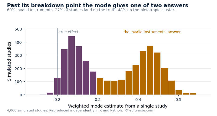
The distribution is not wide. It is bimodal. In 27% of studies the mode landed within 0.05 of the true effect. In 48% it landed above 0.35, on the cluster formed by the invalid instruments. The estimator is not drifting toward a wrong answer as conditions worsen. It is choosing between two answers, and which one it returns depends on the draw.
The interquartile range across replicates makes the same point numerically. At 30% invalid it is 0.016. At 60% invalid it is 0.177, an eleven-fold jump, while the mode’s IQR in every other regime sits between 0.016 and 0.030. Two honest programs disagreeing about the median of that distribution is not a discrepancy to reconcile. It is the correct reading of a quantity that has no stable central value, and it is the same phenomenon we documented when the mean of the ratio estimator failed to converge in our weak-instrument work.
The practical consequence is direct. In this regime a single study produces one mode estimate, with no indication of which peak it came from. A researcher reporting it has roughly a one-in-four chance of reporting the truth and a one-in-two chance of reporting the contamination, and the number itself carries no signal about which happened.
The Failure That No Estimator Catches
Every regime so far has one thing in common: the pleiotropic effects were independent of the instrument strengths. That is the InSIDE assumption, and MR-Egger depends on it entirely. So we broke it. In the final regime the pleiotropic effect on each variant is proportional to that variant’s effect on the exposure, which is what happens when instruments act through a shared upstream biological pathway rather than through unrelated ones.
Against a true effect of 0.200, the four estimators returned 0.298, 0.283, 0.297 and 0.296. Every one of them overstates the effect by roughly 50%. Every one of them agrees with the others to within 0.015. The MR-Egger intercept test fired in 8.3% of studies, statistically indistinguishable from the 7.0% false-positive rate it showed when there was no pleiotropy at all. Cochran’s Q has nothing to find either, because the ratio estimates are not heterogeneous. They are uniformly and consistently wrong.
This is the result that matters most for how MR papers are written. The standard sensitivity block reports four estimates, notes their agreement, and reports a null pleiotropy test. In this regime it produces exactly that output while the causal estimate is inflated by half. Agreement across the four estimators is not evidence that the instruments are valid. It is evidence that the four estimators’ assumptions failed together, or that they all held. The output looks identical either way.
What separates those two possibilities is not more estimators. It is biological argument about the instruments themselves: what genes they sit in, what else those genes do, and whether a shared upstream pathway is plausible. That is what an instrument PheWAS is for, and why Verbanck and colleagues (2018) found detectable horizontal pleiotropy in over 48% of significant causal relationships they tested. It is also why Slob and Burgess (2020), comparing nine robust methods across a wide simulation grid, concluded that no single method dominates and that the choice depends on which violation is plausible for the specific exposure.
Robustness Is Not Free
MR-Egger survived five of our six regimes, which might suggest it should simply be the primary analysis. The precision numbers say otherwise.
| Regime | IVW spread | MR-Egger spread | Egger penalty |
|---|---|---|---|
| No pleiotropy | 0.012 | 0.040 | 3.5x wider |
| Balanced, InSIDE holds | 0.038 | 0.131 | 3.5x wider |
| 30% invalid instruments | 0.019 | 0.127 | 6.5x wider |
Interquartile range of the estimate across 3,000 replicate studies. MR-Egger pays between three and six times the spread of IVW for its robustness, and it carries a small downward bias even when no pleiotropy exists at all, returning 0.190 against a truth of 0.200 in the control condition. An analysis that leads with MR-Egger trades a bias problem for a power problem, which is a real trade and not a free upgrade. Its reliability also depends on the instruments being measured precisely enough, which is what the I-squared-GX statistic of Bowden and colleagues (2016) measures. A low value means the Egger estimate you are leaning on is itself unreliable.
What to Report Instead of “Estimates Were Consistent Across Methods”
The sentence is not wrong, it is just uninformative, because our final regime produces it while the answer is inflated by half. What a methodological reviewer is looking for is different.
- Name the assumption each method buys you. One clause each. IVW assumes all instruments valid, MR-Egger assumes InSIDE, the weighted median assumes under half the weight is invalid, the mode assumes the largest cluster is valid. This tells a reader what your robustness battery actually covers.
- Say which violation you consider plausible for your exposure, and why. This is a biological argument, not a statistical one, and it is the part that distinguishes a considered analysis from a template.
- Report heterogeneity, and act on it. Cochran’s Q with a random-effects IVW model where Q is significant. Our balanced-pleiotropy result shows a fixed-effect interval covering the truth 42.8% of the time while every point estimate looks correct.
- Report the I-squared-GX statistic alongside any MR-Egger estimate. Without it the Egger result cannot be interpreted.
- Run an instrument PheWAS and report what it found. This is the step that addresses the InSIDE-violation regime, and it is the step most submitted MR papers skip.
- Interpret disagreement rather than hiding it. IVW high while the median and mode sit near each other suggests a minority of invalid instruments. All four moving together while Egger’s intercept stays null suggests either clean instruments or a shared pathway, and only biology separates those.
- State instrument strength as well. Everything above assumes strong instruments. Our companion simulation on what the F-statistic actually tells you covers what happens when they are not.
The STROBE-MR statement asks for most of this already. The gap is in what gets done, not in what is documented. Rosas-Chavez and Merriman (2025), evaluating 86 two-sample MR studies of hyperuricaemia and gout published between 2016 and 2024, found that 17% satisfied all three core instrumental-variable assumptions, 14% attempted any replication, and 11% of post-2021 papers complied with STROBE-MR. Our guide to STROBE reporting for observational studies covers the parent guideline, and our overview of causal inference in epidemiology places this design among its alternatives.
Professional Support for a Mendelian Randomization Study
The battery described above is what we run as standard, and the parts that matter most are the ones that address the failure no estimator catches: instrument PheWAS against phenome-wide resources, Steiger filtering, and replication in an independent outcome GWAS. Where the instruments share a plausible upstream pathway, we say so in the manuscript rather than reporting four agreeing numbers and leaving the reader to assume the question was settled.
Feasibility Check
$450
Instrument count, F-statistics, sample overlap and existing literature checked before you commit. Go, modify or stop, in writing. Credited in full against any study you then commission. 5 business days.
Two-Sample MR
$2,900
Full study from public GWAS summary statistics: four estimators, MR-PRESSO, Steiger filtering, instrument PheWAS, leave-one-out, plus a completed STROBE-MR checklist and runnable R code. 15 business days.
Extended Designs
From $3,500
Multivariable MR with conditional F-statistics, mediation MR, colocalisation, drug-target MR and non-linear MR. Fixed quote and written scope before any work begins.
If you are still choosing between a genetic design and a survey, cancer registry or trauma registry analysis, our guide to which health database your study should use sets out what each source can and cannot answer. A robustness battery that agrees across all four estimators still says nothing about whether the study had enough power to detect the effect in the first place, the subject of our companion piece on why Mendelian randomization papers get desk-rejected.
Free Research Tools from Editverse
- GraphPro: build publication-ready charts, 25 types, with built-in t-test, ANOVA, correlation, and chi-square p-values. Free, no signup.
- StatPro: free statistical calculators and a test-selector tool covering group comparisons, categorical outcomes, time-to-event analysis, and diagnostic accuracy.
- Flowchart Pro: generate PRISMA 2020, PRISMA-ScR, CONSORT, STROBE, STARD, MOOSE, and ARRIVE flow diagrams directly in your browser.
Frequently Asked Questions About Pleiotropy in Mendelian Randomization
If all four estimators agree, is my result safe?
No. Agreement is necessary but not sufficient. In our InSIDE-violation regime all four estimators returned values within 0.015 of each other and all four overstated the true effect by roughly 50%, while the MR-Egger intercept test fired at its background false-positive rate. Agreement rules out some failure modes and is silent about others.
Which estimator should be the primary analysis?
Inverse-variance weighting, in almost all cases, with the robust methods as sensitivity analyses. IVW is the most precise by a wide margin, and MR-Egger pays three to six times its spread. Lead with MR-Egger only when you have a specific reason to expect directional pleiotropy, and say what that reason is.
What does it mean when IVW is high but the weighted median and mode are lower?
That pattern is consistent with a minority of strongly invalid instruments, which is exactly the regime the median and mode are built for. It is worth following with MR-PRESSO to identify the outliers and a leave-one-out analysis to confirm no single variant is responsible. Report the analysis both with and without the flagged variants.
Is balanced pleiotropy really harmless?
Not for your confidence interval. In our simulation the IVW point estimate was unbiased under balanced pleiotropy while interval coverage fell from 94.5% to 42.8%. Test for heterogeneity with Cochran’s Q and use a random-effects model where it is significant, otherwise the reported precision is fictional.
What breaks the InSIDE assumption in practice?
Instruments acting through a shared upstream biological pathway, so that a variant with a stronger effect on the exposure also has a proportionally stronger effect through the alternative route. It is most plausible when instruments cluster in genes with related function, and least plausible when they are scattered across unrelated biology. This is a question about your specific instruments, and no statistical test substitutes for looking at them.
How many invalid instruments can the weighted median tolerate?
Up to half the weight, not half the count. Weights depend on instrument strength, so a small number of strong invalid instruments can carry more than half the weight while looking like a minority in the variant table. In our 60%-invalid regime the weighted median returned 0.374 against a truth of 0.200, which is further from the truth than IVW’s 0.367.
Conclusion
Across 72,000 simulated Mendelian randomization estimates, reproduced independently in two programs, the four-estimator sensitivity battery behaved less like a robustness ladder and more like four separate bets. MR-Egger was the only method to survive directional pleiotropy. The weighted median and mode were the only methods to survive a minority of invalid instruments, and the median failed worse than IVW once that minority became a majority. The mode did not degrade past its breakdown point so much as flip between two answers, which is why two honest programs disagreed about its median while matching everywhere else.
The finding worth carrying into a manuscript is the last one. When the InSIDE assumption fails, all four estimators agree with each other, the pleiotropy test reports nothing, and the causal estimate is inflated by half. The output is indistinguishable from a clean analysis. No additional estimator resolves that, because the question is not statistical. It is whether the instruments plausibly reach the outcome through a shared pathway, and answering it means looking at what the genes actually do. A sentence reporting that estimates were consistent across methods is a description of the software output. The reviewer is asking for the argument underneath it.
References
- Bowden J, Davey Smith G, Burgess S. Mendelian randomization with invalid instruments: effect estimation and bias detection through Egger regression. International Journal of Epidemiology. 2015;44(2):512-525. doi:10.1093/ije/dyv080
- Bowden J, Davey Smith G, Haycock PC, Burgess S. Consistent estimation in Mendelian randomization with some invalid instruments using a weighted median estimator. Genetic Epidemiology. 2016;40(4):304-314. doi:10.1002/gepi.21965
- Hartwig FP, Davey Smith G, Bowden J. Robust inference in summary data Mendelian randomization via the zero modal pleiotropy assumption. International Journal of Epidemiology. 2017;46(6):1985-1998. doi:10.1093/ije/dyx102
- Bowden J, Del Greco M F, Minelli C, Davey Smith G, Sheehan NA, Thompson JR. Assessing the suitability of summary data for two-sample Mendelian randomization analyses using MR-Egger regression: the role of the I-squared statistic. International Journal of Epidemiology. 2016;45(6):1961-1974. doi:10.1093/ije/dyw220
- Verbanck M, Chen CY, Neale B, Do R. Detection of widespread horizontal pleiotropy in causal relationships inferred from Mendelian randomization between complex traits and diseases. Nature Genetics. 2018;50(5):693-698. doi:10.1038/s41588-018-0099-7 (PMID 29686387)
- Slob EAW, Burgess S. A comparison of robust Mendelian randomization methods using summary data. Genetic Epidemiology. 2020;44(4):313-329. doi:10.1002/gepi.22295 (PMID 32249995)
- Skrivankova VW, Richmond RC, Woolf BAR, et al. Strengthening the reporting of observational studies in epidemiology using Mendelian randomization: the STROBE-MR statement. JAMA. 2021;326(16):1614-1621. doi:10.1001/jama.2021.18236
- Rosas-Chavez F, Merriman TR. Mendelian randomization studies: a metric for quality evaluation. Gout, Urate, and Crystal Deposition Disease. 2025;3(2):8. doi:10.3390/gucdd3020008 (PMID 42487900)
Simulation details: 30 independent instruments per study; true variant-exposure effects uniform on 0.03 to 0.10 with standard error 0.005; variant-outcome standard error 0.003; true causal effect 0.20; 3,000 replicate studies per regime. Balanced pleiotropy drawn from N(0, 0.010); directional from N(0.006, 0.003); invalid-instrument regimes from N(0.020, 0.005) applied to a random 30% or 60% of variants; InSIDE violation set the pleiotropic effect to 0.10 times each variant’s exposure effect. Weighted mode computed by the Hartwig et al. kernel-density method with bandwidth parameter 1. Implemented independently in R 4.3.3 and Python 3 with NumPy. All reported quantities agreed between engines to within Monte Carlo error except the median weighted mode in the 60%-invalid regime, whose sampling distribution is bimodal and is discussed above.