
The F-statistic is the number a reviewer looks for first in a Mendelian randomization paper, and the rule attached to it, that an instrument is adequate once F exceeds 10, is quoted in almost every methods section written since 2011. Editverse has supported more than 1,100 manuscripts, and in the registry and genetic-epidemiology work our statisticians handle, the F-statistic is also the number authors are most often unable to explain when a reviewer asks what it buys them.
So we measured it. We simulated 135,000 Mendelian randomization studies across a range of instrument strengths and sample-overlap conditions, ran the entire thing twice in two independently written programs, and compared what came out. The result is not the one most tutorials imply. A weak instrument does not usually hand you a wrong answer. It hands you an interval so wide that no answer is possible, and it does so long before the estimate itself starts to drift.
In Simple Words
Think of a genetic instrument as a very small nudge. If the nudge is strong, everyone who carries the variant really does end up with more of the exposure, and you can see what happens to their disease risk. If the nudge is weak, the difference between carriers and non-carriers is barely there, so any effect on disease is buried in noise. The F-statistic measures how strong the nudge is. When it is small, the honest answer your analysis gives back is a range so wide that it includes a large harmful effect, no effect at all, and a large protective effect, all at once. The study has not lied to you. It has simply failed to measure anything.
Where the F Greater Than 10 Rule Came From
The threshold is borrowed, not derived from genetics. It originates in econometrics, where Staiger and Stock (1997) studied two-stage least squares when instruments explain very little of the exposure and proposed a first-stage F of 10 as a working rule of thumb for when the resulting bias is tolerable. The rule crossed into genetic epidemiology through Burgess and Thompson (2011), who examined weak-instrument bias specifically in Mendelian randomization and showed that the estimate is pulled in the direction of the confounded observational association, with the size of the pull governed by the F-statistic.
Two things about that lineage matter and are usually left out. First, the original result concerns two-stage least squares with several instruments, and the bias it describes grows with the number of instruments included. Second, the threshold was offered as a rough guide, not a pass mark. Pierce, Ahsan and VanderWeele (2011) made the related point that instrument strength and statistical power are separate questions, and that an instrument can clear F equals 10 comfortably while leaving a study far too imprecise to answer the question it was built for. Our simulations show exactly how far apart those two things can be. If you are new to the design itself, our guide to what Mendelian randomization is and how to conduct one covers the three instrumental-variable assumptions this article assumes you already know, and our explainer on instrumental variables and two-stage least squares covers the estimator itself.
What We Simulated, and How You Can Check It
The setup is deliberately simple, because a simple design makes the failure mode legible rather than hiding it inside a complicated model. Each simulated study has 5,000 individuals per sample. A single genetic variant with a minor allele frequency of 0.3 acts as the instrument. An unmeasured confounder influences both the exposure and the outcome, which is what makes the observational association misleading in the first place. The true causal effect of the exposure on the outcome is 0.20. Because of the confounder, an ordinary regression of outcome on exposure returns approximately 0.40, so the observational estimate overstates the truth by a factor of two.
We then varied the strength of the instrument so that the first-stage F-statistic landed near 3, 5, 10, 20, 50 and 100, and at each level ran 5,000 replicate studies under two conditions: one where the exposure and outcome associations are estimated in the same participants, and one where they come from two entirely separate samples. For each replicate we recorded the causal estimate, its standard error by the delta method, the resulting 95% confidence interval, and whether that interval contained the true effect of 0.20.
Every figure below was produced twice. One implementation is in R and uses matrix operations over blocks of replicates. The second is in Python and computes the same quantities from sufficient statistics with a different random number generator and no shared code. The two engines were compared before anything was written. They agree on every stable quantity to within Monte Carlo error, and where they disagree, the disagreement is itself the finding. We hold every data figure we publish to this two-engine standard, as in our walkthrough of what NHANES survey weights do and do not fix.
What Weak Instruments Actually Do to the Estimate
The interval collapses long before the point estimate does
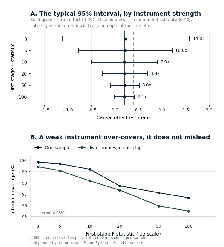
Panel A is the whole argument in one picture. At every instrument strength we tested, the median estimate sits close to the true effect of 0.20 and nowhere near the confounded observational value of 0.40. What changes, dramatically, is the width of the interval around it.
| First-stage F | Median estimate | Median 95% CI width | Width as a multiple of the true effect | Coverage |
|---|---|---|---|---|
| 3 | 0.227 | 2.71 | 13.6x | 99.8% |
| 5 | 0.213 | 1.99 | 10.0x | 99.7% |
| 10 | 0.200 | 1.39 | 7.0x | 99.2% |
| 20 | 0.202 | 0.96 | 4.8x | 97.7% |
| 50 | 0.205 | 0.60 | 3.0x | 97.1% |
| 100 | 0.199 | 0.42 | 2.1x | 96.7% |
Read the fourth column and the practical meaning becomes clear. At an F of 3, the typical confidence interval is 13.6 times wider than the effect the study is trying to detect. That interval stretches from roughly minus 1.1 to plus 1.6. It contains a large protective effect, no effect, and a large harmful effect. Nothing in the data distinguishes between them. At an F of 100 the interval is still about twice the size of the true effect, which is enough to establish a direction but not much more.
The interval width shrinks close to the inverse square root of F. Multiplying each width by the square root of its F gives 4.63, 4.51, 4.37, 4.30, 4.25 and 4.24 across the six levels, which is nearly constant and drifts upward only at the weakest instruments, where the delta-method standard error itself starts to degrade. The practical consequence is that doubling your precision requires roughly quadrupling instrument strength, which in a two-sample design means a far larger exposure GWAS rather than a slightly relaxed p-value threshold.
The interval over-covers, which is not the same as being wrong
Panel B shows coverage: the proportion of replicate studies whose 95% interval contained the true effect. If the method were behaving exactly as advertised, this would sit at 95% everywhere. It does not. At an F of 3 the one-sample interval covered the truth 99.8% of the time, falling to 96.7% at an F of 100. The two-sample intervals track slightly below the one-sample ones and reach 95.5% at the highest strength.
Over-coverage is the signature of a standard error that is too large for the information available. It means a weak instrument produces intervals that are conservative rather than misleading. That is a genuinely important distinction for anyone interpreting a published null result. A Mendelian randomization paper reporting no effect on the basis of a weak instrument has not shown that no effect exists. It has shown that its design could not have detected one. Those are different claims, and reviewers increasingly ask authors to say which one they are making.
The mean does not exist, and two engines proved it
One quantity refused to agree between our two implementations, and the disagreement is instructive. At an F of 3 the R engine returned a mean estimate of 0.64 in the one-sample condition. The Python engine, running the identical design, returned 0.24. In the two-sample condition the two engines returned 0.77 and 1.01. Every other quantity in this article matched to within Monte Carlo error, and these did not.
That is not a bug in either program. The causal estimate here is a ratio of two regression coefficients, and when the denominator can land arbitrarily close to zero, the ratio has no finite expectation. The sample mean of such a quantity does not converge no matter how many replicates you run, so two honest programs will disagree about it indefinitely. The median, the interval width and the coverage all converge normally, which is why the table above reports those and not the mean. Any Mendelian randomization result that leans on an average across variants without acknowledging heavy tails is standing on the same unstable ground, which is one reason the pleiotropy-robust estimators discussed in our main Mendelian randomization guide use medians and modes rather than plain means. Our companion simulation on what each of those four estimators actually protects you from tests them across six pleiotropy regimes and finds one where all four agree and all four are wrong.
Sample Overlap Only Bites When the Instrument Is Weak
Two-sample Mendelian randomization assumes the exposure GWAS and the outcome GWAS were measured in different people. In practice that assumption is violated constantly, because a handful of very large biobanks contribute to a large share of published GWAS, and the same participants turn up on both sides of an analysis without the authors necessarily realising it. Burgess, Davies and Thompson (2016) established that overlap pushes a two-sample estimate back toward the one-sample behaviour, which means back toward the confounded observational association.
We tested the size of that effect directly, varying overlap from 0% to 100% at three instrument strengths.
| Participant overlap | Median bias at F = 3 | Median bias at F = 5 | Median bias at F = 10 |
|---|---|---|---|
| 0% | -0.004 | -0.011 | -0.003 |
| 25% | -0.016 | -0.008 | -0.010 |
| 50% | -0.003 | -0.012 | 0.000 |
| 75% | +0.015 | -0.005 | +0.011 |
| 100% | +0.026 | +0.005 | +0.005 |
At an F of 3 with complete overlap the median estimate is pulled upward by about 0.026 on a true effect of 0.20, a shift of roughly 13% toward the confounded value, and both engines reproduced it independently. At an F of 10 there is no ordered pattern left. The two problems multiply rather than add: overlap converts a weak instrument into a biased one, but on a strong instrument it barely registers.
The reporting implication is direct. Stating that two GWAS overlap is not enough, and neither is asserting that they do not. What a reviewer needs is the overlap fraction alongside the instrument strength, because the first is only interpretable in light of the second. When both are unfavourable, the honest response is not a caveat in the discussion but a different data source.
Why the F Greater Than 10 Rule Still Matters More Than Our Results Suggest
Our simulations use a single instrument, and it would be a serious misreading to conclude from them that weak instruments are harmless. The just-identified case we tested is the friendliest one there is. The bias that Burgess and Thompson (2011) described grows with the number of instruments, so a design with 200 marginally significant variants is exposed to something our single-variant setup cannot show. This is precisely the situation created by relaxing the genome-wide significance threshold from 5 x 10 to the minus 8 down to 1 x 10 to the minus 5 in order to obtain more instruments, which is now common practice for exposures with sparse genetic architecture.
Two further points belong in any honest treatment. In multivariable Mendelian randomization the relevant quantity is not the ordinary F-statistic at all but the conditional F-statistic introduced by Sanderson and colleagues (2019), which measures whether the instruments can distinguish the exposures from one another rather than merely predicting each in isolation. Papers routinely report the wrong statistic here. Separately, when instruments are measured with error the MR-Egger estimate becomes unreliable, and the diagnostic for that is the I-squared-GX statistic of Bowden and colleagues (2016). A low value means the sensitivity analysis you were relying on to defend against pleiotropy is itself not trustworthy.
What Reviewers Actually Find in Published MR Papers
The gap between the standard described above and the standard applied in practice has now been measured. Rosas-Chavez and Merriman (2025) systematically evaluated 86 two-sample Mendelian randomization studies of hyperuricaemia and gout published between 2016 and 2024, scoring each against a structured quality metric. Their findings, in their own numbers:
- 66% satisfied the relevance assumption, meaning genome-wide significance or a reported F-statistic above 10. One paper in three did not.
- 51% used datasets with no participant overlap, which by their own reporting leaves roughly half the literature exposed to the interaction described above.
- 59% addressed statistical power at all.
- 17% satisfied all three core instrumental-variable assumptions.
- 14% conducted any replication analysis.
- 11% of papers published after 2021 complied with the STROBE-MR reporting guideline.
Overall quality scores in that review ranged from 0 to 19 on a scale running to 21, with a mean of 9.1. This is one disease area, and other fields may differ, but it is the most systematic audit of MR reporting quality currently available and the direction it points in matches what our own statisticians see in submitted manuscripts. When five papers in six fail to satisfy the assumptions their own conclusions depend on, editors respond by raising the bar for everyone, which is why methodological completeness has become a gatekeeping issue rather than a stylistic one. Our guide to STROBE reporting for observational studies covers the parent guideline that STROBE-MR extends.
How to Report Instrument Strength So a Reviewer Can Check It
Reporting a single number and moving on is what generates the query. The following is what our statisticians put in a methods section, and what a methodological reviewer is looking for when they open one.
- Per-instrument and combined F-statistics. Report both. A combined F of 40 built from thirty variants each with an F near 1.3 is a different object from a combined F of 40 built from three strong variants, and only the per-variant table shows which you have.
- The proportion of exposure variance explained. State the R-squared for the instrument set. This is what determines precision, and it is the quantity a reader needs in order to judge whether your interval could ever have been narrow enough to be useful.
- The selection threshold, stated before the results. If you relaxed below genome-wide significance, say so, say why, and report the analysis at both thresholds so a reader can see whether the finding depends on the relaxation.
- The clumping parameters and reference panel. Linkage-disequilibrium threshold, window size, and which panel was used. Instruments that are not independent inflate apparent strength.
- The overlap fraction, with its source. Name the cohorts contributing to each GWAS and estimate the shared proportion. If you cannot estimate it, say that, and treat the analysis as a one-sample design for interpretation.
- A precision statement, not only a significance statement. Report the minimum effect size your design could have detected. A null result without this is uninterpretable, as the coverage results above show.
- The conditional F-statistic for any multivariable analysis. The ordinary F does not answer the question multivariable Mendelian randomization asks.
Three Mistakes That Produce This Failure
Treating F greater than 10 as a pass mark rather than a floor. Clearing 10 does not make a study adequate. On our numbers an F of 10 still leaves an interval seven times wider than the effect being measured. The threshold marks the point below which bias becomes a concern, not the point above which precision becomes sufficient.
Relaxing the p-value threshold to obtain more instruments. This is the single most common route into weak-instrument territory, and it does the opposite of what the author intends. It adds variants that contribute little strength while increasing the instrument count, which is the combination the classic bias result warns about. If an exposure has too few genome-wide significant variants, that is information about whether the study should proceed, not an obstacle to be worked around.
Reporting a null as evidence of no effect. With a weak instrument the interval covers the truth 99.8% of the time precisely because it covers almost everything. A null from an underpowered design is a statement about the design, and reviewers who understand this will say so. Our guide to levels of evidence in clinical research covers where a well-executed MR result sits relative to trial evidence, and our overview of causal inference in epidemiology covers the broader family of designs this one belongs to. A null result from a weak-instrument design is also uninterpretable on its own, which is the subject of our companion piece on why Mendelian randomization papers get desk-rejected.
Professional Support for a Mendelian Randomization Study
Instrument strength is the first thing our statisticians check, and it is checked before any analysis is commissioned rather than reported afterwards. If an exposure has too few independent genome-wide significant variants, or if the only available outcome GWAS shares a substantial sample with the exposure GWAS, we say so at the outset. The alternative is producing a technically correct analysis that no reviewer will accept and no reader can use.
Feasibility Check
$450
Instrument count, F-statistics, sample overlap and existing literature checked before you commit. Go, modify or stop, in writing. Credited in full against any study you then commission. 5 business days.
Two-Sample MR
$2,900
Full study from public GWAS summary statistics: four estimators, MR-PRESSO, Steiger filtering, instrument PheWAS, leave-one-out, plus a completed STROBE-MR checklist and runnable R code. 15 business days.
Extended Designs
From $3,500
Multivariable MR with conditional F-statistics, mediation MR, colocalisation, drug-target MR and non-linear MR. Fixed quote and written scope before any work begins.
If you are still choosing between a genetic design and a survey, cancer registry or trauma registry analysis, our guide to which health database your study should use sets out what each source can and cannot answer.
Free Research Tools from Editverse
- GraphPro: build publication-ready charts, 25 types, with built-in t-test, ANOVA, correlation, and chi-square p-values. Free, no signup.
- StatPro: free statistical calculators and a test-selector tool covering group comparisons, categorical outcomes, time-to-event analysis, and diagnostic accuracy.
- Flowchart Pro: generate PRISMA 2020, PRISMA-ScR, CONSORT, STROBE, STARD, MOOSE, and ARRIVE flow diagrams directly in your browser.
Frequently Asked Questions About Instrument Strength in Mendelian Randomization
Is an F-statistic above 10 enough for publication?
It is necessary, not sufficient. Our simulations show that at an F of 10 the typical 95% interval is still seven times wider than the effect being estimated, which is enough to establish that the design is not badly biased and not enough to answer most research questions. Reviewers increasingly expect a precision statement alongside the F-statistic, showing the smallest effect the study could have detected.
How do I calculate the F-statistic for multiple instruments?
For a set of independent variants the combined F can be computed from the total proportion of exposure variance explained and the sample size, using F equal to R-squared times the quantity n minus k minus 1, divided by the quantity 1 minus R-squared, times k, where k is the number of instruments. Report the per-variant F-statistics as well, because a high combined value can be produced either by a few strong instruments or by many weak ones, and only the former is reassuring.
Does weak-instrument bias push toward the null or toward the confounded estimate?
It depends on the design. In a one-sample analysis the bias is toward the confounded observational association. In a genuinely two-sample analysis with no participant overlap it is toward the null. Partial overlap sits between the two, which is why the overlap fraction has to be reported alongside the instrument strength rather than instead of it.
Can I relax the p-value threshold to get more instruments?
You can, but it usually makes the problem worse rather than better. Variants selected at a relaxed threshold add little to the proportion of exposure variance explained while increasing the number of instruments, and weak-instrument bias in the over-identified case grows with instrument count. If you do relax the threshold, report the analysis at both thresholds so a reader can see whether the result survives.
What if my exposure has only a handful of genome-wide significant variants?
Then the honest answer may be that a Mendelian randomization study is not the right design for that exposure yet. The interval will be wide enough to include almost anything, and neither the estimate nor a null result from it will be interpretable. This is a question worth settling before the analysis rather than after, which is what a feasibility assessment is for.
How do I know whether two GWAS share participants?
Read the contributing cohort lists in each publication and its supplementary material. Very large biobanks appear in a substantial share of published GWAS, so the default assumption for any two large studies of a common trait should be that some overlap exists until you have checked. Where the overlap cannot be quantified, interpret the analysis as a one-sample design.
Conclusion
Across 135,000 simulated Mendelian randomization studies, reproduced independently in two programs, the F-statistic turned out to govern something other than what it is usually invoked for. The median estimate stayed close to the truth at every instrument strength we tested. What changed by a factor of six was the width of the interval around it, from 2.1 times the true effect at an F of 100 to 13.6 times at an F of 3. Sample overlap only produced a detectable shift where the instrument was already weak, and even then the shift was small next to the imprecision surrounding it.
The practical reading is that instrument strength is a question about whether a study can answer anything, and only secondarily a question about bias. That reframing changes when the check should happen. An F-statistic reported in a results table is a description of a study that has already been run. An F-statistic calculated during design is a decision about whether to run it. Given that only 17% of the papers in the most systematic published audit satisfied all three core assumptions, and only 14% attempted replication, the checks that happen before the analysis are the ones that separate a manuscript that clears review from one that does not.
References
- Staiger D, Stock JH. Instrumental variables regression with weak instruments. Econometrica. 1997;65(3):557-586. doi:10.2307/2171753
- Burgess S, Thompson SG. Avoiding bias from weak instruments in Mendelian randomization studies. International Journal of Epidemiology. 2011;40(3):755-764. doi:10.1093/ije/dyr036 (PMID 21414999)
- Pierce BL, Ahsan H, VanderWeele TJ. Power and instrument strength requirements for Mendelian randomization studies using multiple genetic variants. International Journal of Epidemiology. 2011;40(3):740-752. doi:10.1093/ije/dyq151 (PMID 20813862)
- Burgess S, Davies NM, Thompson SG. Bias due to participant overlap in two-sample Mendelian randomization. Genetic Epidemiology. 2016;40(7):597-608. doi:10.1002/gepi.21998
- Bowden J, Del Greco M F, Minelli C, Davey Smith G, Sheehan NA, Thompson JR. Assessing the suitability of summary data for two-sample Mendelian randomization analyses using MR-Egger regression: the role of the I-squared statistic. International Journal of Epidemiology. 2016;45(6):1961-1974. doi:10.1093/ije/dyw220
- Sanderson E, Davey Smith G, Windmeijer F, Bowden J. An examination of multivariable Mendelian randomization in the single-sample and two-sample summary data settings. International Journal of Epidemiology. 2019;48(3):713-727. doi:10.1093/ije/dyy262
- Rosas-Chavez F, Merriman TR. Mendelian randomization studies: a metric for quality evaluation. Gout, Urate, and Crystal Deposition Disease. 2025;3(2):8. doi:10.3390/gucdd3020008 (PMID 42487900)
- Skrivankova VW, Richmond RC, Woolf BAR, et al. Strengthening the reporting of observational studies in epidemiology using Mendelian randomization: the STROBE-MR statement. JAMA. 2021;326(16):1614-1621. doi:10.1001/jama.2021.18236
Simulation details: 5,000 individuals per sample, single biallelic instrument at minor allele frequency 0.3, unmeasured confounder loading 0.5 on both exposure and outcome, true causal effect 0.20, confounded observational association 0.40. Instrument strength calibrated to target first-stage F values of 3, 5, 10, 20, 50 and 100. 5,000 replicates per cell. Implemented independently in R 4.3.3 and Python 3 with NumPy; all reported quantities agreed between engines to within Monte Carlo error except the mean of the ratio estimator, which has no finite expectation and is discussed above.