
Reviewers read your figures before they read your methods. The clinical research graphs that survive peer review share one trait: each one answers a single question, and the reader can see the answer in under ten seconds. This guide covers the 10 plots a clinical researcher meets most often, from the CONSORT flow diagram to the heatmap. For each one you get a real published figure (open access, reused with attribution), our own animated illustration, how to read it, and the mistake that gets manuscripts sent back.
In Simple Words
A graph is an answer to a question. “Who was in the trial?” is a flow diagram. “How long did patients live?” is a survival curve. “Do two machines agree?” is a Bland-Altman plot. Pick the graph by the question, not by what looks impressive.
Pick Clinical Research Graphs by the Question
| Your question | Graph | Typical study |
|---|---|---|
| Who was screened, randomised, analysed? | CONSORT flow diagram | Randomised trial |
| How long until the event? | Kaplan-Meier curve | Cohort, trial |
| What do many studies say together? | Forest plot | Meta-analysis |
| Are small studies missing? | Funnel plot | Meta-analysis |
| Does a test separate sick from well? | ROC curve | Diagnostic accuracy |
| Do two methods agree? | Bland-Altman plot | Method comparison |
| How did each patient’s tumour respond? | Waterfall plot | Oncology phase II |
| Which of thousands of genes changed? | Volcano plot | Omics, biomarkers |
| What does the whole distribution look like? | Violin or box plot | Any group comparison |
| How do many variables relate or tune? | Heatmap | Correlation, parameter sweeps |
That companion guide, 10 Essential Graph Types Every Researcher Should Know, covers general chart types such as bar, line, scatter and histogram. This post is different: it covers only the plots specific to trials, diagnostic tests and evidence synthesis.
1. CONSORT Flow Diagram: Show Every Patient
The flow diagram is the first figure a trial reviewer checks. It answers who was screened, who was excluded and why, who was randomised, and who ended up in the analysis. The CONSORT 2010 statement makes it a required item for randomised trials.1
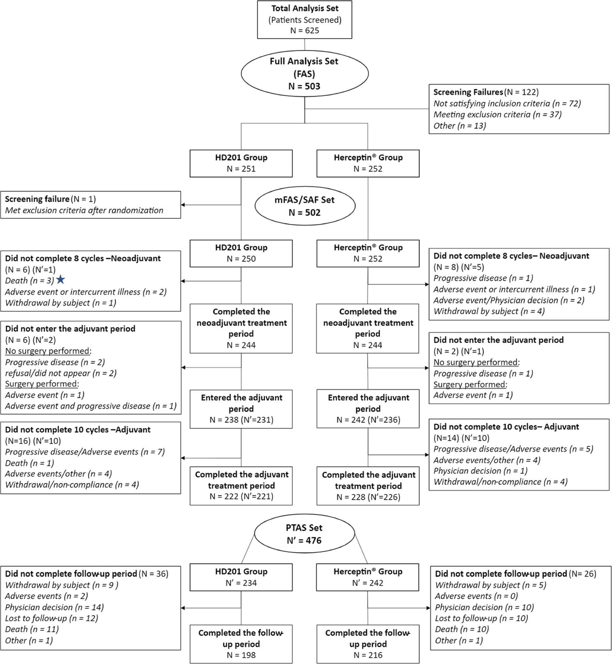
In this randomised comparison of the trastuzumab biosimilar candidate HD201 with reference trastuzumab in neoadjuvant ERBB2-positive breast cancer, 625 patients were screened and 503 entered the full analysis set: 251 on HD201 and 252 on the reference product.2 A reader can check the arithmetic at a glance, which is exactly the point.
Common mistake: boxes with counts but no reasons. “Excluded (n = 122)” invites a query. Say how many failed each criterion. You can build the diagram free in the Flowchart Pro generator.
2. Kaplan-Meier Curve: Time to Event, Honestly Drawn
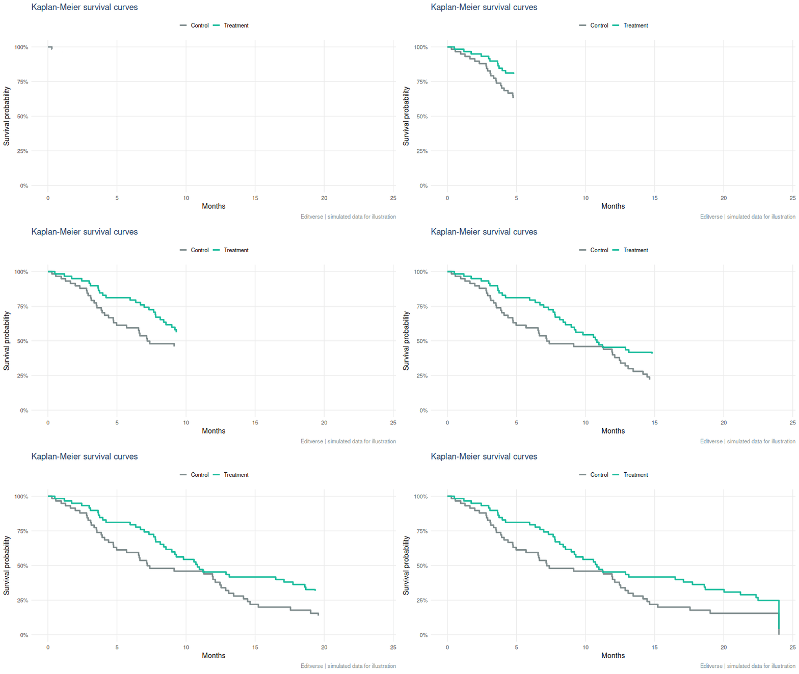
The Kaplan-Meier estimator turns follow-up times, including patients who have not yet had the event, into a stepped survival curve.3 Read the drop of each step as events, and the small tick marks as patients who left follow-up event-free (censored).
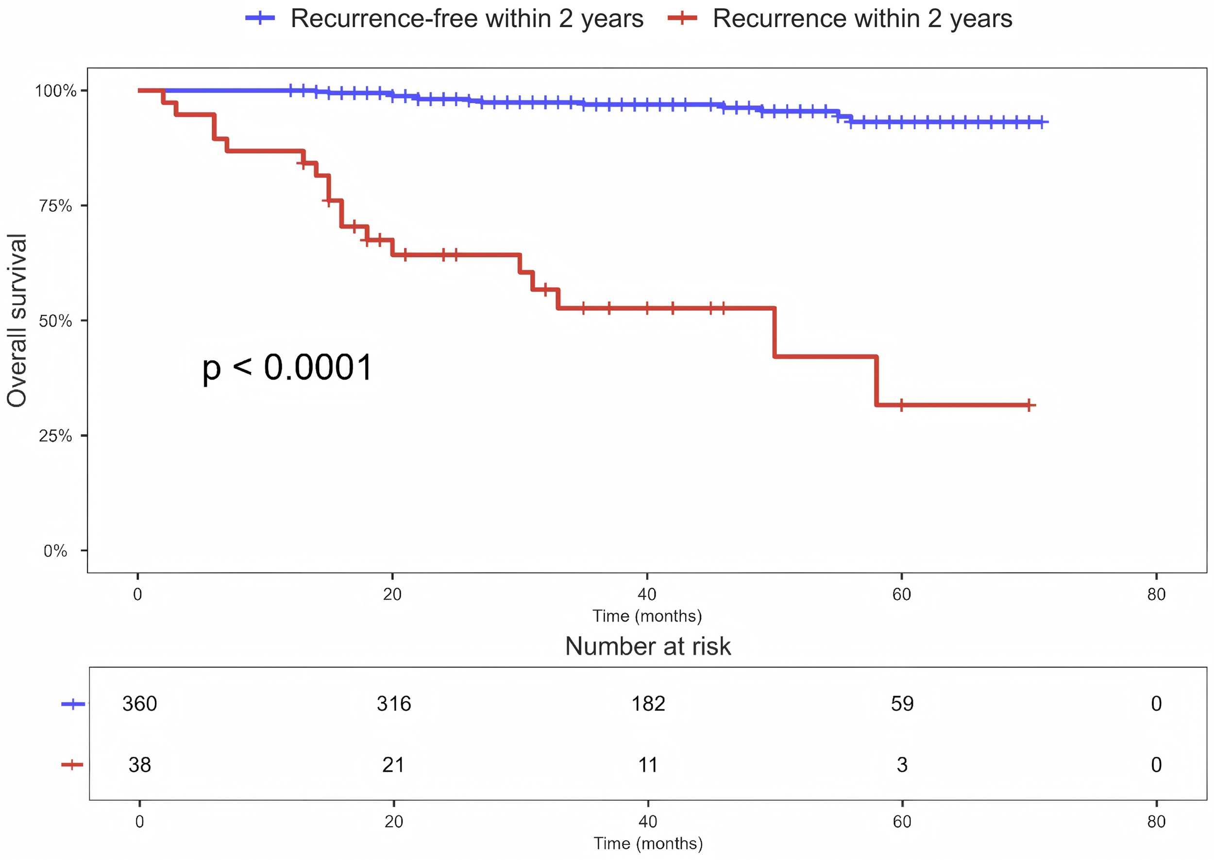
Read the real example the way a reviewer would.12 Patients who recurred within 2 years (red) fall to about 32% survival by month 58, while those recurrence-free (blue) stay above 90%. The table underneath is the honest part: the red group starts with 38 patients and has 3 left at 60 months, so the far right of that curve rests on very few people. Always draw that table, and treat steps in a thinly populated tail as soft.
How to make it reviewer-proof: print a number-at-risk table under the x-axis, state the median follow-up, give the hazard ratio with its 95% confidence interval next to the log-rank p-value, and stop interpreting the curve where very few patients remain at risk. If patients can die of something else before your event, the plain curve overstates risk; see competing risks in registry studies. To try it on your own data, use the free Kaplan-Meier calculator.
3. Forest Plot: Many Studies, One Verdict
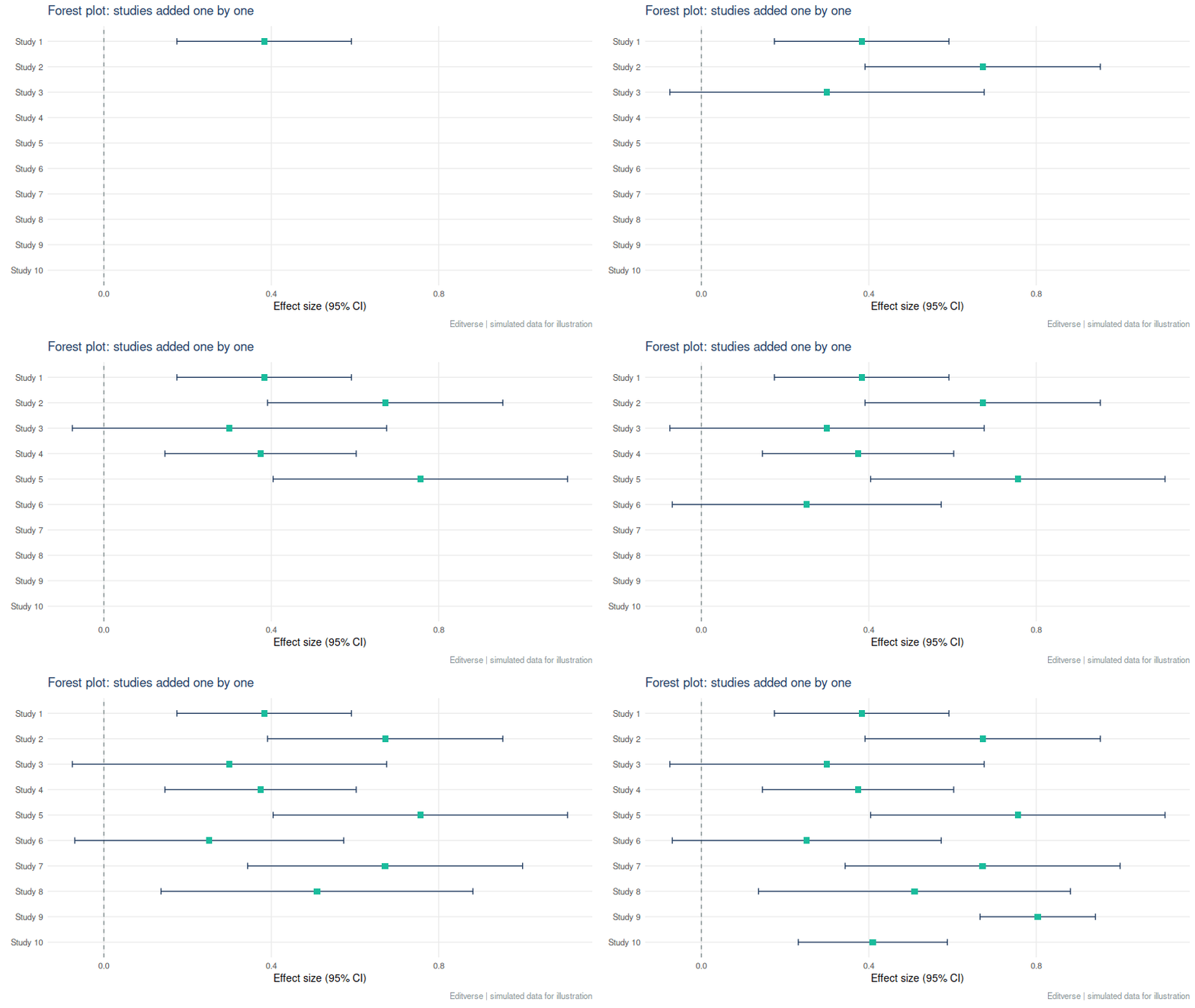
A forest plot lists each study as a square (its effect) with a line (its confidence interval), then a diamond for the pooled result. Squares scale with weight, so large studies pull the diamond harder.

This one reports a pooled adjusted odds ratio of 3.28 (95% CI 2.61 to 4.12) with I² = 95.4%.4 The lesson sits in that second number. I² describes the share of variation that is real between-study difference rather than chance.5 At 95.4% the single pooled figure hides a lot. Report a prediction interval, explore the reasons (subgroups, meta-regression), and word the conclusion as “associated with higher odds in most settings”, not as one fixed number.
Planning one? Read how many studies a meta-analysis needs and the common mistakes in meta-analysis. The logistic regression calculator also draws an odds-ratio forest plot.
4. Funnel Plot: Where Are the Small Studies?
A funnel plot sets each study’s effect against its precision. Without bias, studies scatter symmetrically around the pooled effect, wide at the bottom (small studies) and narrow at the top. A bite missing from one lower corner suggests small null studies never reached print.
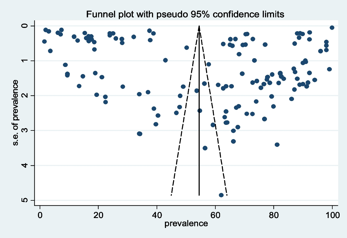
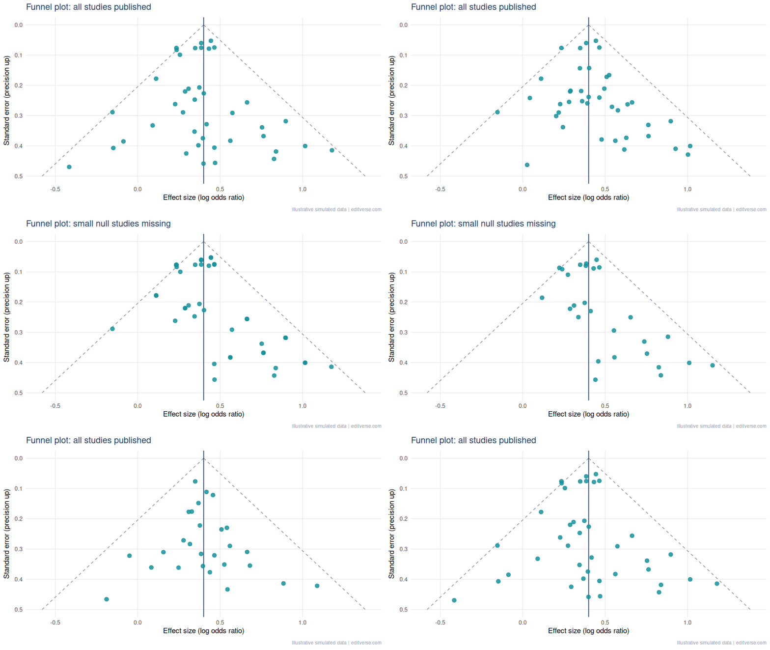
Rule of thumb: test for asymmetry (Egger’s test6) only with about 10 or more studies, and never treat asymmetry as proof of bias. Heterogeneity produces the same shape.
5. ROC Curve: Can the Test Tell Sick from Well?
The ROC curve plots sensitivity against 1 minus specificity across every possible cut-off. The area under it (AUC) is the chance that a random patient with the disease scores higher than a random patient without it. 0.5 is a coin flip, 1.0 is perfect.7
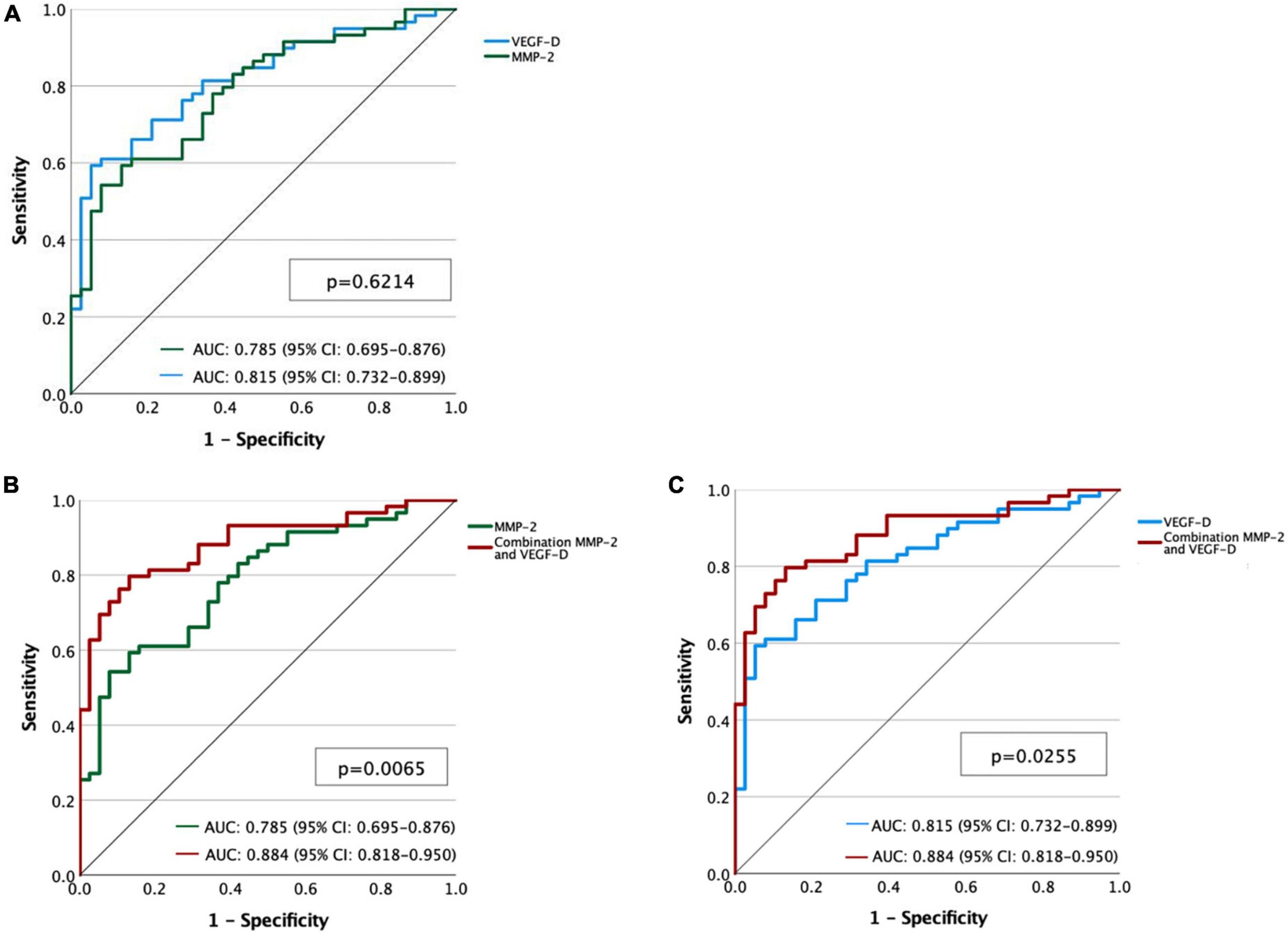
Here the AUCs are 0.785 for MMP-2, 0.815 for VEGF-D and 0.884 for the combination.8 A worked reading: combining the two markers lifts discrimination by about 0.07 to 0.10 AUC over either alone, which is a meaningful gain, but only if the confidence intervals do not overlap heavily and the model is checked on new patients.
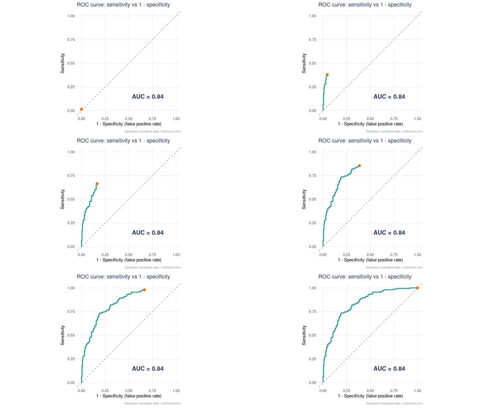
Common mistake: reporting AUC alone. Also give the chosen cut-off, its sensitivity and specificity with confidence intervals, and say how you chose it (Youden index, or a clinical cost trade-off). An AUC says nothing about whether a test is useful at the bedside.
6. Bland-Altman Plot: Agreement Is Not Correlation
When you compare two measurement methods, a high correlation only says they rise and fall together. It does not say they give the same number. The Bland-Altman plot graphs the difference between methods against their mean, with the average difference (bias) and limits of agreement at bias ± 1.96 SD.9
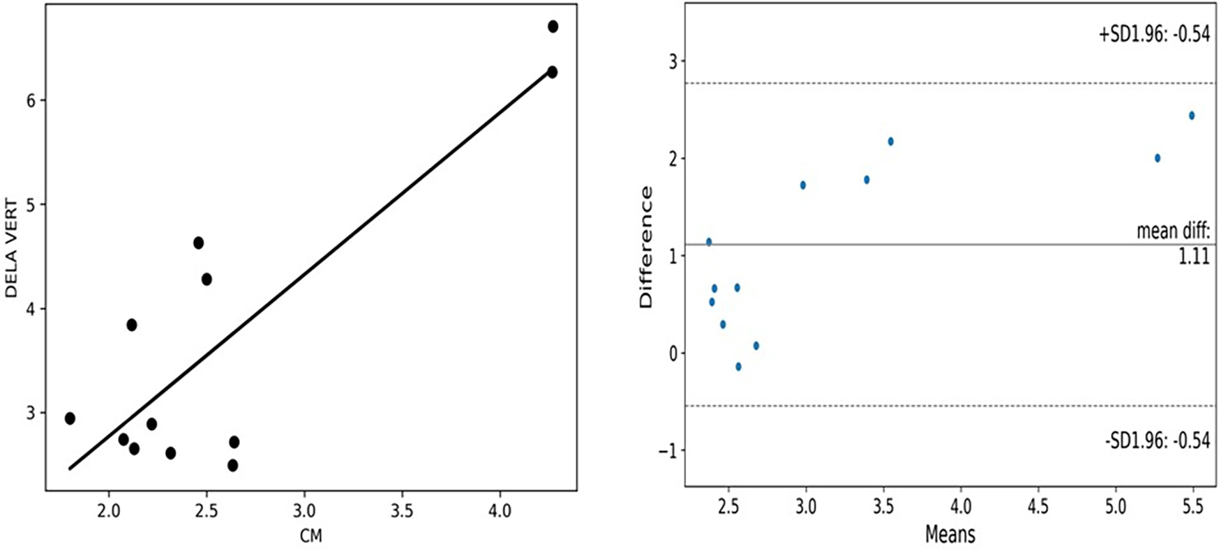
This figure from a lower-limb oedema feasibility study teaches two things.10 The mean difference is 1.11, and the plotted limits run from about -0.54 to 2.77. And the differences climb as the mean rises, a proportional bias. The left panel looks like decent agreement because the points follow a line. The right panel shows the methods disagree, and by more at higher values. That gap is why reviewers ask for this plot.
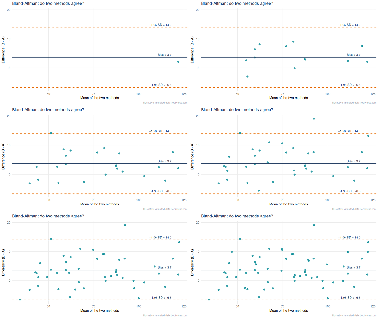
A pattern we see when editing method-comparison manuscripts: a correlation coefficient presented as proof of agreement, with no Bland-Altman plot. Add the plot, state the bias and limits in the units of measurement, and say in one sentence whether those limits are clinically acceptable. The clinical judgement, not the statistics, decides that.
7. Waterfall Plot: Every Patient’s Tumour Response
A waterfall plot gives each patient one bar: the best percentage change in tumour size from baseline, sorted from worst to best. Under RECIST 1.1, a 30% decrease counts as a partial response and a 20% increase as progression, so those two reference lines belong on the plot.11
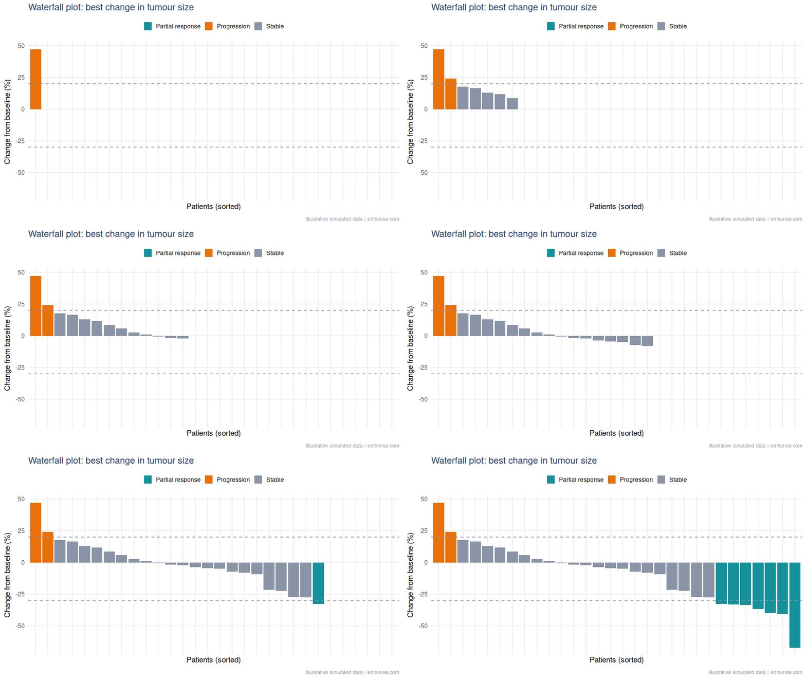
Common mistake: using it to imply duration. A waterfall shows the best response, not how long it lasted. Pair it with a swimmer plot or a time-to-progression curve, and say how many patients had no post-baseline scan, since they cannot appear as bars.
8. Volcano Plot: Find the Signal Among Thousands
A volcano plot puts effect size on the x-axis (log2 fold change) and significance on the y-axis (minus log10 of the p-value). Genes that are both large and significant sit in the top corners. It turns a table of thousands of rows into one picture.
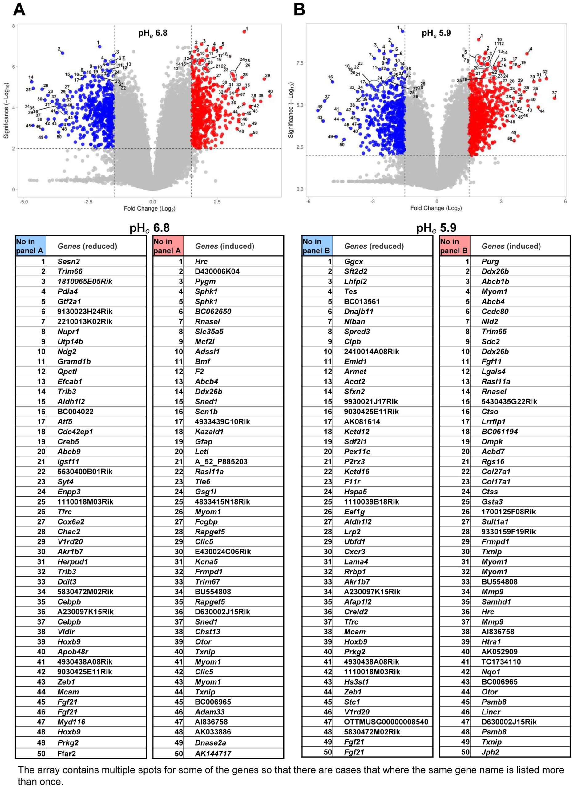

Common mistake: colouring points by raw p-value after testing thousands of genes. Colour by the adjusted value (false discovery rate), state both thresholds in the caption, and name only the few genes you discuss in the text.
9. Violin and Box Plots: Show the Whole Distribution
A bar of means hides everything a clinician cares about: spread, skew, outliers, and whether groups overlap. A box plot shows the median and quartiles. A violin adds the shape of the distribution, which matters when values are skewed or bimodal.
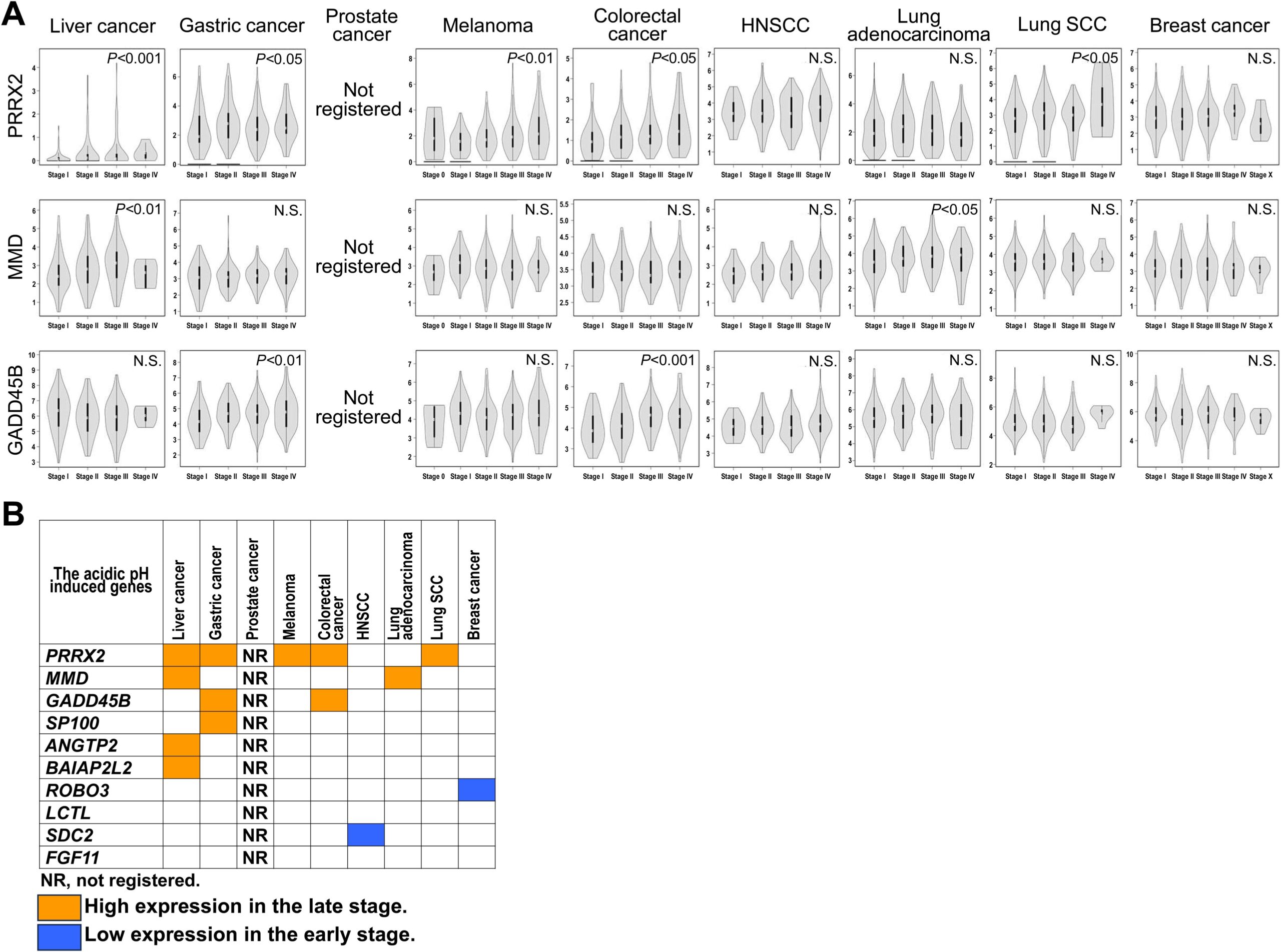
Rule: overlay the raw points whenever each group has fewer than about 30 patients. Small samples make violin shapes unreliable, and individual dots let the reader judge for themselves. Our general-chart guide covers box plots and histograms in more detail.
10. Heatmap: Patterns Across Many Variables
A heatmap colours a grid. Clinical papers use it for correlation matrices, gene-expression clusters and parameter sweeps. Print the number in each cell if the grid is small enough to read.
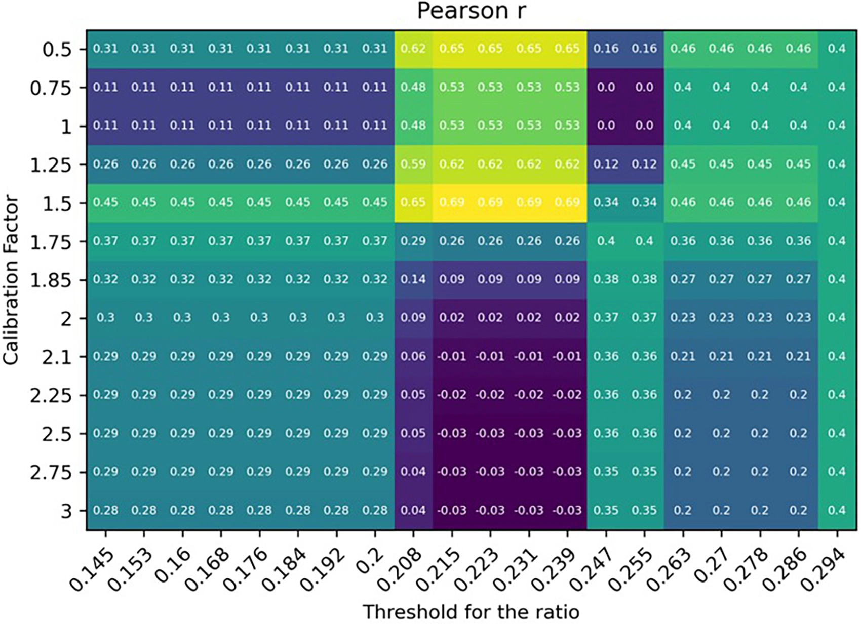
In this sweep, r peaks at 0.69 at a calibration factor of 1.5, while some cells fall to zero or below.10 It is a good teaching case: the best cell was picked from the same data it was scored on, so 0.69 is an optimistic figure until checked on new patients. A heatmap that tunes parameters should always say so.
Colour tip: use a perceptually uniform, colour-blind-safe scale (viridis is the usual choice, as in this figure), and never a red-green scale.
The 60-Second Figure Checklist for Clinical Manuscripts
- One graph, one question. Say the question in the caption.
- Units, sample size and the statistical test appear on or under every figure.
- Uncertainty (confidence interval, IQR or SD) is always visible.
- Text is readable at single-column width, which is about 8.5 cm in most journals.
- Colours survive greyscale printing and colour-blind readers.
- Reused figures carry their licence and a full citation.
Free Research Tools from Editverse
- GraphPro: build publication-ready charts, 25 types, with built-in t-test, ANOVA, correlation, and chi-square p-values. Free, no signup.
- StatPro: free statistical calculators and a test-selector tool covering group comparisons, categorical outcomes, time-to-event analysis, and diagnostic accuracy.
- Flowchart Pro: generate PRISMA 2020, PRISMA-ScR, CONSORT, STROBE, STARD, MOOSE, and ARRIVE flow diagrams directly in your browser.
Professional Statistical and Figure Support for Your Clinical Manuscript
Choosing the right graph is half the job. Running the analysis behind it correctly, and drawing it to a journal’s specification, is the other half. If you are a PhD student, clinician or busy investigator with data in hand and a deadline, these three services cover the path from dataset to submission-ready figure.
Figures
$300
Data Visualization Service. Up to 10 forest plots, survival curves, ROC curves and heat maps, formatted to your target journal. 3-5 business days.
Analysis and review
$475
Statistical Analysis & Review Services. A PhD biostatistician reviews or runs your analysis and writes the statistical methods section. 5-10 business days, 60 days of revisions.
Complex methods
$750
Advanced Statistical Analysis. Cox regression, mixed models, propensity score matching and multivariate methods. 5-7 business days.
Running a full evidence synthesis instead? See our meta-analysis and systematic review service, and for a quick sanity check on a result, Statistical Results Interpretation.
Clinical Research Graphs: Frequently Asked Questions
Which graph shows survival data?
A Kaplan-Meier curve, drawn with censor marks and a number-at-risk table beneath it. Report the hazard ratio with its 95% confidence interval alongside the log-rank p value.
Is a high correlation enough to show two methods agree?
No. Correlation shows that two methods rise and fall together, not that they give the same number. A Bland-Altman plot shows the bias and the limits of agreement in the units you measured.
What does an AUC of 0.8 mean on an ROC curve?
It means a randomly chosen patient with the disease scores higher on the test than a randomly chosen patient without it about 80% of the time. It does not say whether the test is useful at the bedside, so also report the cut-off with its sensitivity and specificity.
When should I draw a funnel plot?
In a meta-analysis with about 10 or more studies. With fewer, the plot and Egger’s test are unreliable. Asymmetry can come from heterogeneity as well as publication bias.
Can I reuse a figure from a published paper in my manuscript?
Only if its licence allows it. Figures under CC BY can be reused with full attribution. Otherwise ask the publisher for permission or rebuild the graph from the reported numbers and cite the source.
Conclusion: Choosing Clinical Research Graphs
Ten graphs cover most of what a clinical paper needs: a flow diagram to account for patients, a survival curve for time to event, forest and funnel plots to pool and stress-test evidence, ROC and Bland-Altman plots to judge tests and measurements, a waterfall for tumour response, a volcano for omics, a violin for distributions, and a heatmap for patterns. Choose by the question, show the uncertainty, and put the numbers a reviewer will look for in the caption. If you want a second pair of eyes on your figures before submission, our team can help.
References
- Schulz KF, Altman DG, Moher D; CONSORT Group. CONSORT 2010 statement: updated guidelines for reporting parallel group randomised trials. BMJ. 2010;340:c332. doi:10.1136/bmj.c332
- Pivot X, Manikhas AG, Shamrai V, et al. Final analysis of the phase 3 randomized clinical trial comparing HD201 vs. referent trastuzumab in patients with ERBB2-positive breast cancer treated in the neoadjuvant setting. BMC Cancer. 2023;23:112. doi:10.1186/s12885-023-10574-2
- Kaplan EL, Meier P. Nonparametric estimation from incomplete observations. J Am Stat Assoc. 1958;53(282):457-81. doi:10.1080/01621459.1958.10501452
- Ayenew AA, Mol BW, Bradford B, Abeje G. Prevalence of female genital mutilation and associated factors among women and girls in Africa: a systematic review and meta-analysis. Syst Rev. 2024;13:26. doi:10.1186/s13643-023-02428-6
- Higgins JPT, Thompson SG, Deeks JJ, Altman DG. Measuring inconsistency in meta-analyses. BMJ. 2003;327(7414):557-60. doi:10.1136/bmj.327.7414.557
- Egger M, Davey Smith G, Schneider M, Minder C. Bias in meta-analysis detected by a simple, graphical test. BMJ. 1997;315(7109):629-34. doi:10.1136/bmj.315.7109.629
- Hanley JA, McNeil BJ. The meaning and use of the area under a receiver operating characteristic (ROC) curve. Radiology. 1982;143(1):29-36. doi:10.1148/radiology.143.1.7063747
- Revilla-López E, Ruiz de Miguel V, López-Meseguer M, et al. Lymphangioleiomyomatosis: searching for potential biomarkers. Front Med. 2023;10:1079317. doi:10.3389/fmed.2023.1079317
- Bland JM, Altman DG. Statistical methods for assessing agreement between two methods of clinical measurement. Lancet. 1986;1(8476):307-10. doi:10.1016/S0140-6736(86)90837-8
- Lippi L, et al. Three-dimensional laser scanning technology for accurate lower limb edema assessment in heart failure patients: a feasibility study. Front Cardiovasc Med. 2026. doi:10.3389/fcvm.2026.1750128
- Eisenhauer EA, et al. New response evaluation criteria in solid tumours: revised RECIST guideline (version 1.1). Eur J Cancer. 2009;45(2):228-47. doi:10.1016/j.ejca.2008.10.026
- Liu C, Zhou J, Lam W, Wang C, et al. Prognostic value of initial recurrence pattern for post-recurrence survival in locally advanced rectal cancer after neoadjuvant chemoradiotherapy and surgery. Front Oncol. 2026;16:1836607. doi:10.3389/fonc.2026.1836607
- Kato Y, Mawatari K. Clinical significance of acidic extracellular microenvironment modulated genes. Front Oncol. 2024;14:1380679. doi:10.3389/fonc.2024.1380679
Figures marked CC BY 4.0 are reproduced under the Creative Commons Attribution licence with the original authors credited. Animated illustrations use simulated data and are original to Editverse.