
Published
A Mendelian randomization power calculation is the one step in the whole pipeline that costs nothing to run and gets skipped anyway. Rosas-Chavez and Merriman audited 86 two-sample MR studies of hyperuricaemia and gout published between 2016 and 2024 and found that 59 percent addressed power at all, which means 41 percent reported a causal estimate, positive or null, with no statement of whether the study could have detected the effect it was looking for (Gout, Urate, and Crystal Deposition Disease 2025;3(2):8, doi:10.3390/gucdd3020008). A null result from an underpowered design and a null result from a genuinely absent effect look identical on the page. Only a power calculation tells a reader which one they are reading.
This piece is the third simulation in our Mendelian randomization series, and it closes a loop the first two opened. Our piece on what the F-statistic actually tells you showed that a weak instrument inflates the width of the confidence interval rather than the point estimate. Our piece on what each of the four estimators protects you from showed that pleiotropy can make four different methods agree on the same wrong answer. Neither post answered a plainer question a reviewer asks before either of those diagnostics is even relevant. Given the instrument you actually have and the outcome sample you actually have, could your study have found the effect you are claiming to test for. We built a two-sample Mendelian randomization power model, validated it independently in Python and R, and ran it across the range of study sizes that appear in the published literature.
In Simple Words
Before running a Mendelian randomization study, you can work out in advance how likely it is to detect a real effect, the same way a clinical trial calculates how many patients it needs. Two numbers mostly decide the answer, how many people are in the outcome dataset and how much of the exposure your genetic instrument actually explains. Many published MR studies use a modest case-control outcome sample and a single genetic variant, which is a combination that misses a real but moderate effect more often than it finds it. When that happens, the paper reports a null result as though the exposure has no causal effect, when the honest reading is that the study was never able to tell either way.
What Reviewers Actually Check Now
Mendelian randomization moved from a specialist method to a reviewer checklist item over roughly a decade, and the checklist has three parts. Skrivankova and colleagues formalised it as the STROBE-MR statement, a 20-item extension of STROBE built specifically for genetic instrumental variable studies and co-published in the BMJ and JAMA (JAMA 2021;326(16):1614-1621, doi:10.1001/jama.2021.18236). Item 7 asks authors to describe how they assessed their assumptions, and the elaboration document names the F-statistic explicitly as the tool for judging instrument strength, the subject of our first spoke. Item 4b asks something separate. It requires authors to report the sample size and state whether a power or sample size calculation was carried out before the main analysis, noting that power is best read from the width of the 95 percent confidence interval once the study is complete (BMJ 2021;375:n2233, doi:10.1136/bmj.n2233).
The gout and hyperuricaemia audit is the only quantified check we could find of how often that item is actually satisfied, and the pattern across all three checks is consistent rather than reassuring. Sixty-six percent of the 86 studies met the relevance assumption on instrument strength, 51 percent used non-overlapping exposure and outcome samples, 59 percent addressed power, and only 17 percent satisfied all three core instrumental variable assumptions at once. Eleven percent of the post-2021 papers complied with STROBE-MR in full. A study can therefore report a strong F-statistic, a clean single-sample design and still be silent on whether it had any chance of detecting the effect its abstract discusses.
The Formula Behind a Mendelian Randomization Power Calculation
Brion, Shakhbazov and Visscher supplied the framework the field still uses. Working from asymptotic theory for a continuous exposure and a single genetic predictor, they showed that statistical power at a fixed sample size reduces to two quantities, the proportion of variance in the exposure that the instrument explains and the true causal effect being tested (International Journal of Epidemiology 2013;42(5):1497-1501, doi:10.1093/ije/dyt179). Burgess extended the approach to binary outcomes and worked sample size in the other direction, from a target power back to the N a study would need (International Journal of Epidemiology 2014;43(3):922-929, doi:10.1093/ije/dyu005).
For the two-sample design that almost every current MR study actually runs, exposure and outcome associations estimated in separate GWAS samples, the standard error of the ratio estimate is set mostly by the outcome sample, because the exposure GWAS behind a well-studied trait is usually far larger and its first-stage estimate correspondingly more precise. For standardised exposure and outcome variables, the approximate standard error of the causal estimate scales as one divided by the square root of the outcome sample size multiplied by the instrument’s R squared. A weak instrument and a small outcome sample fail the same way, they both shrink that product, and the noncentrality parameter behind the power calculation is the true effect multiplied by the square root of that same quantity. Reporting the F-statistic and reporting power are answering the same underlying question from two different angles, which is exactly why STROBE-MR asks for both.
How We Tested It
We built the closed-form Mendelian randomization power calculation above and checked it against three independent sources of evidence, following the same validation gate as our earlier two spokes. First, we cross-checked a fast, vectorised simulation that draws each replicate’s SNP-exposure and SNP-outcome estimates directly from their sampling distributions against a slow simulation that generates individual-level genotypes, exposures and outcomes and runs the actual regressions, on three parameter combinations. Both agreed within Monte Carlo error at a few hundred replicates. Second, we ran the full grid twice, once in Python with NumPy and once independently in R, at 200,000 replicates per cell, using different random number generators and no shared code. Third, we compared both simulated engines against the closed-form formula itself. The delta-method standard error for the two-sample Wald ratio, which propagates uncertainty from both the SNP-exposure and SNP-outcome estimates rather than treating the instrument as known exactly, follows Burgess, Butterworth and Thompson’s summarised-data framework (Genetic Epidemiology 2013;37(7):658-665, doi:10.1002/gepi.21758).
Every cell in both experiments below agreed across all three checks to within a percentage point or two of simulated power, which at 200,000 replicates is tighter than the Monte Carlo noise floor. Scripts and results are available on request. Agreement held across the parameter range that matters for a real study design, so the closed form is trustworthy there, and the rest of this post reports simulated values, which make no simplifying assumption about a perfectly known instrument.
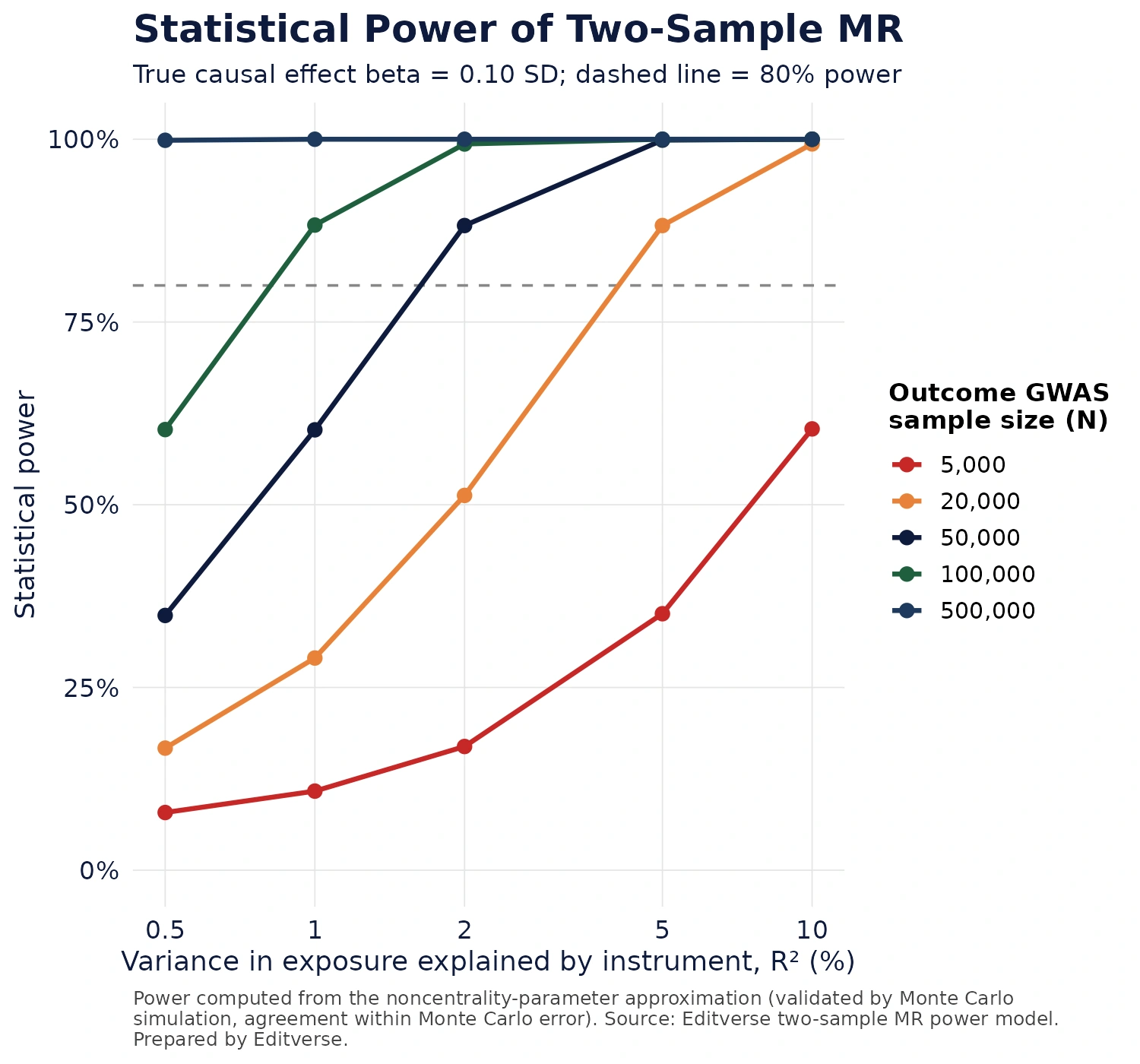
Reading the surface confirms the formula’s shape rather than anything surprising in isolation, and that is the point of validating one. At an outcome sample of 500,000, the study range most large biobank analyses now use, power clears 99 percent even at the smallest instrument strength on the grid. At an outcome sample of 5,000, a size still common for a case-control study of a less common outcome, power does not reach 80 percent anywhere on the R squared axis we tested, topping out at 60 percent even when a single instrument explains a generous 10 percent of exposure variance. Between those extremes the two axes trade off directly. An outcome sample of 20,000 needs an instrument explaining roughly 4 to 5 percent of exposure variance to reach conventional power, a threshold few single-SNP instruments clear and that usually requires pooling several genome-wide-significant variants into a polygenic score.
Six Designs, One Effect Size
A grid over abstract parameters is a model check. What a reviewer wants to know is whether a design that looks ordinary in a submitted manuscript was ever capable of finding what it claims to have found. We built six study designs spanning the published range of two-sample MR, a small case-control outcome with a single lead SNP, a mid-sized cohort outcome with either a single SNP or a pooled multi-SNP score, and a large biobank outcome across three instrument strengths, then computed power for each at three true effect sizes, a modest 0.05 SD, a moderate 0.10 SD, and a large 0.20 SD.
| Design | Outcome N / R² | Power at beta=0.05 | Power at beta=0.10 | Power at beta=0.20 |
|---|---|---|---|---|
| Small case-control, single lead SNP | 4,000 / 0.5% | 5.5% | 7.3% | 14.1% |
| Mid cohort, single lead SNP | 25,000 / 0.8% | 10.7% | 29.3% | 79.1% |
| Mid cohort, multi-SNP instrument | 25,000 / 2% | 19.9% | 60.4% | 99.2% |
| Large biobank, single lead SNP | 400,000 / 0.5% | 60.8% | 99.4% | 100% |
| Large biobank, multi-SNP instrument | 400,000 / 3% | 99.98% | 100% | 100% |
| Large biobank, well-powered exposure | 400,000 / 8% | 100% | 100% | 100% |
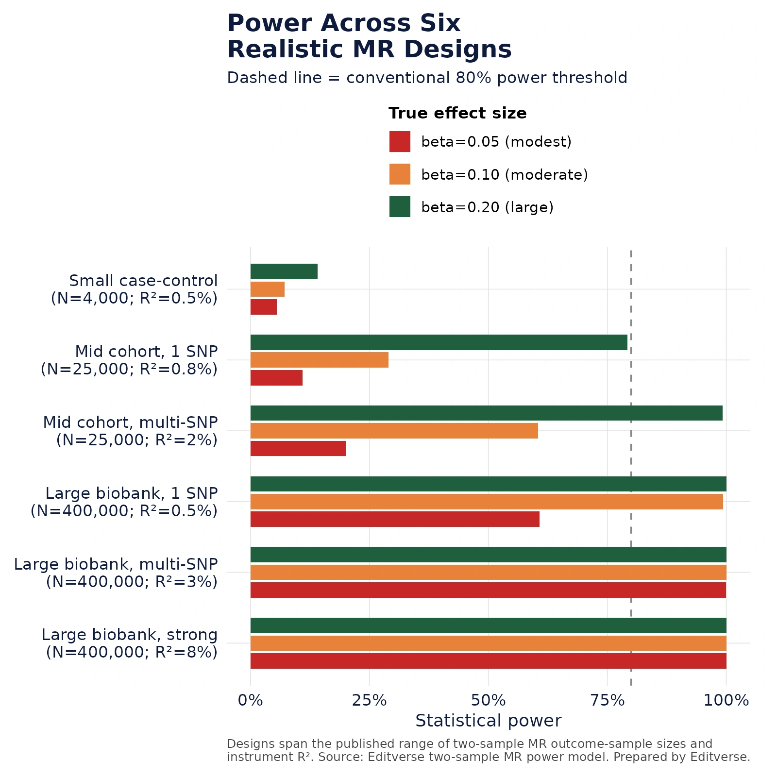
Two of the six designs never reach conventional power for a moderate effect, and a third barely does. A small case-control outcome stays under 15 percent power even for a large 0.20 SD effect, which means a null finding from that design is close to uninformative regardless of what the true causal relationship happens to be. The mid-sized cohort with a single lead SNP needs the effect to be large before power crosses 80 percent, and most exposures of applied interest, a modest change in a biomarker or an inflammatory marker, are not expected to move an outcome by a large margin. Only the two large-biobank designs with a pooled multi-SNP instrument clear 80 percent power even at the smallest effect size tested, which is also the combination that has become standard in disease areas with enormous genome-wide association study resources, such as lipids, blood pressure and body mass index, and far rarer in less-studied exposures.
Why an Underpowered Null Still Gets Published as a Real Finding
Absence of evidence is treated as evidence of absence more often in Mendelian randomization than the method allows for, because the ratio estimate is not obviously any less certain-looking when it comes from an underpowered study than when it comes from a well-powered one. A cause-specific hazard ratio from a small cohort at least carries a visibly wide confidence interval that a reader can eyeball. A null MR estimate with a moderate confidence interval reads as a clean answer even when the study never had a realistic chance of rejecting the null for the effect size that would actually matter clinically.
This is the mechanism behind the 41 percent of studies in the Rosas-Chavez and Merriman audit that said nothing about power. Once a paper reports a point estimate near zero and a confidence interval that crosses it, the manuscript reads as complete without a power statement, and neither the authors nor, evidently, most reviewers ask the next question, whether the study was ever positioned to see an effect of a size that would be biologically or clinically relevant. STROBE-MR item 4b exists specifically to close that gap, asking authors to state up front whether a power calculation was carried out, and the explanation document is blunt that the confidence interval width after the fact is itself the most honest indicator of what the study could support.
A practical fix costs one paragraph and one number. Before commissioning or submitting an MR analysis, run a Mendelian randomization power calculation for the minimum detectable effect at 80 percent power given the instrument’s known R squared and the outcome sample’s known size, using the same noncentrality-parameter approach behind Figure 1, then state that number in the methods alongside the F-statistic. A null result reported next to a minimum detectable effect of 0.03 SD is a real finding. A null result reported next to a minimum detectable effect of 0.25 SD, next to a literature that suggests the true effect if it exists is closer to 0.10 SD, is a design limitation dressed as a conclusion.
The Tension With the Other Two Spokes
Raising power by adding more genetic variants to the instrument is the obvious response to a small R squared, and it interacts with the other two failure modes in this series rather than sidestepping them. Every additional SNP pooled into a score raises R squared and therefore power, which is good for the concern in this post, but each additional variant is also an additional opportunity for horizontal pleiotropy, the failure mode our second spoke quantified, where a shared upstream pathway can move all four common estimators toward the same wrong answer while looking like agreement. A large, powerful instrument is not automatically a valid one, and the pleiotropy diagnostics from that post do not become less necessary as the instrument grows.
Weak-instrument bias relates to power in the opposite direction. Our first spoke found that a low first-stage F-statistic inflates the width of the confidence interval without shifting the median point estimate in the just-identified case, which sounds like it would only ever produce an honest null rather than a false positive. Combine that with the finding here, and the honest null from a weak instrument is frequently also an underpowered null, which means the same design flaw that widens the interval also lowers the chance of detecting a real effect at all. A paper can report a wide, correctly centred, non-significant interval from a weak single-SNP instrument and be simultaneously technically unbiased and practically unable to answer its own research question. This is the third time in this series that a method behaving exactly as its statistical theory predicts still produces a misleading paper, because the theory describes what the estimator does and says nothing about whether the design gave it enough information to work with.
Free Research Tools from Editverse
- GraphPro: build publication-ready charts, 25 types, with built-in t-test, ANOVA, correlation, and chi-square p-values. Free, no signup.
- StatPro: free statistical calculators and a test-selector tool covering group comparisons, categorical outcomes, time-to-event analysis, and diagnostic accuracy.
- Flowchart Pro: generate PRISMA 2020, PRISMA-ScR, CONSORT, STROBE, STARD, MOOSE, and ARRIVE flow diagrams directly in your browser.
Professional Support for a Mendelian Randomization Study
A power calculation belongs at the design stage, not the response-to-reviewers stage, because a study that turns out to be underpowered after the data are in hand cannot be fixed by writing a better discussion section. Our biostatisticians run the instrument-strength and power calculations before any analysis begins, report a minimum detectable effect alongside every null result, and check the instrument against pleiotropy diagnostics from more than one estimator, following the STROBE-MR checklist item by item rather than retrofitting it after a reviewer asks.
Feasibility Check
$450
Whether a usable instrument exists for your exposure, what its likely R squared is against public GWAS resources, and a minimum detectable effect at your available outcome sample size before you commit to the full study. Credited in full against any study you then commission. 5 business days.
Two-Sample MR Study
$2,900
Full causal analysis with F-statistic, power and minimum detectable effect reported alongside the estimate, pleiotropy checked across IVW, MR-Egger, weighted median and weighted mode, MR-PRESSO and Steiger filtering applied, plus manuscript, figures and a completed STROBE-MR checklist. Public GWAS summary statistics, we obtain them. 15 business days.
Extended Designs
From $3,500
Multivariable MR across correlated exposures, bidirectional and Steiger-filtered designs, instrument PheWAS against candidate pleiotropic pathways, and joint power calculations across two or more exposures analysed together. Fixed quote and written scope before any work begins.
The pillar behind this series, Mendelian randomization explained, covers the full method from instrument selection through to reporting, and our walkthrough of instrumental variable approaches sets out the statistical machinery a power calculation is built on. If you are still deciding whether MR is the right design for your question, which health database your study should use compares it against registry and survey designs, and our guide to levels of evidence in clinical research sets out where a well-powered causal design like this one sits relative to trial evidence.
Conclusion
A Mendelian randomization power calculation is not a formality to add after the analysis runs. It determines whether the paper’s central claim, positive or null, is a finding about the exposure or a finding about the study’s own sample size. Our validated model puts a number on the two quantities that decide it, the outcome sample and the instrument’s R squared, and the six realistic designs we tested show that a sizeable share of the study shapes still common in the literature, a modest cohort outcome paired with a single lead variant, do not reach conventional power for an effect most researchers would consider worth reporting.
None of the three spokes in this series describes a broken method. The F-statistic, the four pleiotropy-robust estimators and the power calculation all do exactly what their statistical theory says they do. What they share is that none of them substitutes for the other two, and a paper that reports only one, an F-statistic above 10 with no power statement, or a clean null with no minimum detectable effect, has satisfied the letter of the STROBE-MR checklist without answering the question a careful reviewer is actually asking. Reporting all three costs a short paragraph. Leaving one out is how a design limitation becomes a published conclusion.
References
- Brion MJA, Shakhbazov K, Visscher PM. Calculating statistical power in Mendelian randomization studies. Int J Epidemiol. 2013;42(5):1497-1501. doi:10.1093/ije/dyt179
- Burgess S. Sample size and power calculations in Mendelian randomization with a single instrumental variable and a binary outcome. Int J Epidemiol. 2014;43(3):922-929. doi:10.1093/ije/dyu005
- Burgess S, Butterworth A, Thompson SG. Mendelian randomization analysis with multiple genetic variants using summarized data. Genet Epidemiol. 2013;37(7):658-665. doi:10.1002/gepi.21758
- Skrivankova VW, Richmond RC, Woolf BAR, et al. Strengthening the Reporting of Observational Studies in Epidemiology Using Mendelian Randomization: the STROBE-MR statement. JAMA. 2021;326(16):1614-1621. doi:10.1001/jama.2021.18236
- Skrivankova VW, Richmond RC, Woolf BAR, et al. Strengthening the reporting of observational studies in epidemiology using Mendelian randomisation (STROBE-MR): explanation and elaboration. BMJ. 2021;375:n2233. doi:10.1136/bmj.n2233
- Rosas-Chavez F, Merriman TR. Mendelian randomization studies: a metric for quality evaluation. Gout Urate Crystal Deposition Dis. 2025;3(2):8. doi:10.3390/gucdd3020008