Migliori bar chart vs histogram question comes down to one thing: what is on the horizontal axis. This guide gives the rule, then shows what goes wrong when it is broken, using real data: 272 eruptions of the Old Faithful geyser, drawn first as a bar chart and then as a histogram. The bar chart says the typical eruption lasts about 3.5 minutes. The histogram shows that very few eruptions do.
Su questa pagina: La differenza · Esempio pratico · Bin width · What journals show · Errore comune · Quale usare · Costruisci entrambi · FAQ
Bar chart vs histogram: the difference in one table
Both charts use bars, which is why they get confused. The difference is the type of variable on the horizontal axis. A grafico a barre has categories: treatment arms, hospitals, diagnoses. Each bar is its own thing, so there is a gap between bars and the order is free. A istogramma has one continuous measurement, such as age, a lab value or a duration. The measurement is cut into consecutive bins and each bar counts the observations in one bin, so the bars touch and the order is fixed.
| Caratteristica | Grafico a barre | Istogramma |
|---|---|---|
| What the horizontal axis shows | Separate categories (groups, diagnoses, countries) | One continuous measurement cut into consecutive bins |
| What the bar height shows | A count, a percentage or a summary such as a mean | The number (or share) of observations in that bin |
| Spazi tra le barre | Yes, to mark separate categories | No, bars touch because the scale is continuous |
| Can you reorder the bars? | Yes, for example from largest to smallest | No, the number line fixes the order |
| Choice you must make | Which categories to show | Where the bins start and how wide they are |
| Domanda tipica a cui viene data risposta | Which group is larger? | What shape does the distribution have: one peak, two peaks, skew, gaps? |
Our practical advice: when in doubt, ask whether you could swap two bars without changing the meaning. If you can, it is a bar chart. If swapping would scramble the number line, it is a histogram.
Worked example: 272 geyser eruptions, drawn two ways
R ships a dataset called faithful with 272 observations of the Old Faithful geyser in Yellowstone, originally analysed by Azzalini and Bowman [5]. We took the eruption durations in minutes. The mean is 3.49 minutes, the standard deviation 1.14, the median 4.0, and the range 1.6 to 5.1. We recomputed these in both R and Python from the same file and the results agree.
Figure 1 draws the same 272 numbers twice. Panel A is the bar chart a lot of papers would print: one bar at the mean with an error bar of one standard deviation. Panel B is the histogram.

faithful dataset, 272 eruptions [5]; plot by Editverse.Panel A tells you “eruptions last about 3.5 minutes, give or take a minute.” Panel B shows that is wrong as a description of any single eruption. There are two clusters: short eruptions near 2 minutes and long ones near 4.5 minutes. Of the 272 eruptions, 97 (36%) last under 3 minutes and 175 (64%) last 3 minutes or more. Only 14 eruptions (5%) fall between 2.5 and 3.5 minutes, and just 17 (6%) are within a quarter of a minute of the mean. The bar chart’s mean, and the error bar around it, describe a duration that the geyser rarely produces.
This is the core reason to prefer a histogram for continuous data: a summary bar can come from very different distributions, and only a histogram (or a dot plot) shows which one you have.
How bin width changes what a histogram says
A histogram has a setting a bar chart does not: the bin width. Figure 2 shows the same data with four widths.
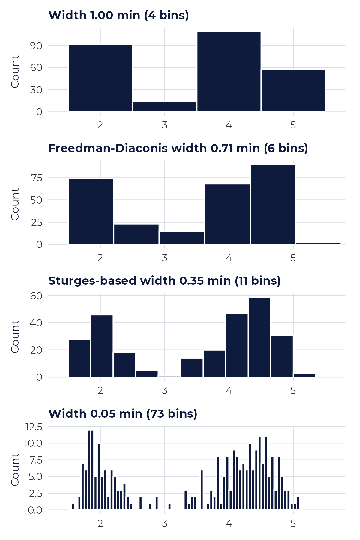
faithful dataset [5]; plot by Editverse.| Bin width | Bins drawn | Da dove viene | What you would conclude |
|---|---|---|---|
| 1.00 min | 4 | A round number | Two big blocks and a small one; the dip is there, but the shape is crude |
| 0.71 min | 6 | Freedman-Diaconis rule [4] | The two clusters are visible, with two low bins between them |
| 0.35 min | 11 (rule gives 10 classes) | Sturges rule [2] | Two clear clusters and an almost empty gap between them |
| 0.05 min | 73 | Arbitrario | Jagged; single bins look like peaks, which is mostly noise |
Three published rules give a starting point. Sturges (1926) uses k = ceil(log2 n) + 1 classes, which is 10 for n = 272 [2]. Scott (1979) gives a width of 3.49 x SD x n^(-1/3), which is 0.61 minute here [3]. Freedman and Diaconis (1981) use 2 x IQR x n^(-1/3), which is 0.71 minute here and is less affected by outliers [4]. These are rules of thumb, not laws. Our advice is to try two or three widths, check that the story does not change, and state the bin width or rule in the figure legend.
One detail that trips people up: whether bins are open on the left or the right decides where a value that sits exactly on an edge is counted. R’s hist e closed = "right" setting we used count a value of 4.0 in the bin (3.75, 4.0]. Software defaults differ, so say which you used when the counts matter.
What published figures actually show
The habit of drawing a bar for a mean is widespread. Weissgerber and colleagues reviewed research articles in top physiology journals (n = 703) and found that 85.6% included at least one bar graph. Most of these showed mean plus or minus the standard error (77.6%) rather than the standard deviation (15.3%). Figures that show the distribution were seldom used: 13.4% of articles had at least one univariate scatterplot, 5.3% a box plot and 8.0% a histogram [1].
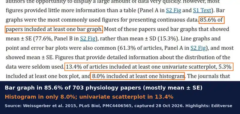
The authors’ point, in the abstract, is that many different data distributions can lead to the same bar or line graph, and that the full data may suggest different conclusions from the summary statistics [1]. That is exactly what Figure 1 shows with a single dataset. The review dates from 2015, so it describes practice in that period, but it remains the clearest audit of the problem.
Common mistake: a bar chart of the mean for a continuous variable
Three related slips are worth checking in your own figures:
- Touching bars for categories, or gaps for bins. The gap is a signal: it says “these are separate groups”. Use it correctly.
- Error bars that do not say what they are. Standard error shrinks as the sample grows and is not a description of spread. State SD or SE in the legend, and prefer showing the points [1].
- Bin width chosen by the software default and never checked. As Figure 2 shows, the same data can look blocky or jagged depending on one setting.
Quale grafico dovresti usare?
- Comparing groups on a count or share (cases per hospital, proportion with each outcome): bar chart, y-axis starting at zero.
- Looking at the shape of one continuous measurement (age, biomarker, duration): histogram, with the bin width stated.
- Comparing a continuous outcome between a few groups: show the individual points, or box plots, or one histogram per group on a shared axis; a bar of the mean is the last choice [1].
- Two continuous variables: a scatterplot rather than either bar form.
For more on choosing, see our guides to scegliere il tipo di grafico giusto and how graph choice changes data interpretation, and for the test that goes with your chart, scegliere il test statistico giusto.
How to build both charts in R
The code below reproduces Figure 1 in a few lines. It uses the built-in dataset, so you can run it as is.
library(ggplot2)x <- faithful$eruptions # 272 Old Faithful eruptions, minutes# 1. the bar chart of the mean (hides the shape)mean(x); sd(x) # 3.49, 1.14# 2. the histogram (shows the shape); bins are (a, b], right-closedggplot(faithful, aes(eruptions)) + geom_histogram(breaks = seq(1.5, 5.5, by = 0.25), closed = "right", fill = "#0F1B3D", colour = "white") + geom_vline(xintercept = mean(x), linetype = "dashed", colour = "#c62828")# 3. bin-width rules from base R: number of classes each rule suggestsnclass.Sturges(x); nclass.scott(x); nclass.FD(x)
You can also make histograms and bar charts without code with our free tool below.
Free tools for your charts
Questi strumenti di Editverse sono gratuiti e non richiedono registrazione.
- GraphProCrea grafici pronti per la pubblicazione, di 25 tipologie diverse, con test t, ANOVA, correlazione e valori p del chi-quadrato integrati. Gratuito, senza registrazione.
- StatiProCalcolatori statistici gratuiti e uno strumento di selezione dei test che copre confronti tra gruppi, risultati categorici, analisi del tempo all'evento e accuratezza diagnostica.
- Flowchart Pro: Genera diagrammi di flusso PRISMA 2020, PRISMA-ScR, CONSORT, STROBE, STARD, MOOSE e ARRIVE direttamente nel tuo browser.
Guide correlate di Editverse
Get your figures built to journal standard
If you want your data drawn as the right chart, with the distribution visible and the legend and format set for your target journal, this is the service built for it.

Need figures that show your real data? We turn your data into publication-ready charts built to your target journal’s specification: histograms, scatter and dot plots, box and violin plots, forest plots and more, in R (ggplot2), with revisions until they match the journal’s requirements.
Bar chart vs histogram FAQ
What is the difference between a bar chart and a histogram?
A bar chart compares separate categories, so its bars are spaced apart and can be reordered. A histogram shows how one continuous measurement is distributed: the values are cut into consecutive bins, the bars touch, and the order is fixed by the number line.
When should I use a bar chart instead of a histogram?
Use a bar chart when the horizontal axis lists categories, such as treatment groups, hospitals or diagnoses, and the bar height is a count, a percentage or a summary value. Use a histogram when the horizontal axis is a measured quantity, such as age, blood pressure or eruption time.
Why do the bars in a histogram touch each other?
Because the bins are consecutive intervals on a continuous scale, with no gap between the end of one interval and the start of the next. A gap between bars would suggest a break in the scale. A gap in a bar chart marks the separation between unrelated categories.
Is a bar chart of means a good way to show continuous data?
Often not. In a review of 703 articles in top physiology journals, 85.6% included at least one bar graph, and the authors warn that many different data distributions can lead to the same bar graph [1]. Our Old Faithful example below shows a mean of 3.49 minutes where very few eruptions last that long.
Quanti intervalli dovrebbe avere un istogramma?
There is no single correct number. Sturges’ rule uses k = ceil(log2 n) + 1 classes, Scott’s rule a width of 3.49 x SD x n^(-1/3), and Freedman and Diaconis a width of 2 x IQR x n^(-1/3) [2,3,4]. For the 272 eruptions these give 10 classes (width 0.35 min), a width of 0.61 min and a width of 0.71 min. Try more than one setting and report the one you used.
Can a histogram hide a feature of my data?
Yes. Too few bins smooth away real structure, and too many bins draw noise. With four bins of 1 minute the two clusters of Old Faithful eruptions blur into a blocky shape; with 73 bins of 0.05 minute the pattern turns jagged.
Should the y-axis of a bar chart start at zero?
Yes. In a bar chart the length of the bar carries the value, so cutting off the bottom exaggerates differences. This rule is for bars; a histogram’s y-axis is a count of observations and should also start at zero, because bar height is again the message.
What should I show instead of a bar graph of means in a small study?
Show the individual data points, for example a univariate scatterplot, or a box plot or histogram when the sample is large enough. Weissgerber and colleagues found that these were rare in physiology papers: 13.4% had a scatterplot, 5.3% a box plot and 8.0% a histogram [1].
Conclusione
Use a bar chart when the horizontal axis lists categories and a histogram when it is a number line. For continuous data, a bar of the mean can hide structure that a histogram reveals: in our 272 eruptions the mean describes a duration the geyser rarely produces. State your bin width, say whether your error bars are SD or SE, and when the sample is small show every point [1,2,3,4]. For help turning your data into the right figure, see our servizio di visualizzazione dei dati.
Referenze
- Weissgerber TL, Milic NM, Winham SJ, Garovic VD (2015). Beyond bar and line graphs: time for a new data presentation paradigm. PLoS Biol 13(4):e1002128. 10.1371 / journal.pbio.1002128
- Sturges HA (1926). The choice of a class interval. J Am Stat Assoc 21(153):65-66. 10.1080/01621459.1926.10502161
- Scott DW (1979). On optimal and data-based histograms. Biometrika 66(3):605-610. 10.1093/biomet/66.3.605
- Freedman D, Diaconis P (1981). On the histogram as a density estimator: L2 theory. Z Wahrscheinlichkeitstheorie verw Gebiete 57(4):453-476. 10.1007 / BF01025868
- Azzalini A, Bowman AW (1990). A look at some data on the Old Faithful geyser. Appl Stat 39(3):357-365. 10.2307/2347385
faithful dataset, and the cited figures and statements were checked against the source papers on 28 October 2026.