Propensity Matching Clinical Research: Python Tutorial
Master propensity matching clinical research with Python. Learn treatment effects, covariate balance, and real-world applications with comprehensive examples.
Table of Contents
- Introduction to Propensity Matching Clinical Research
- Clinical Datasets for Propensity Matching Clinical Research
- Propensity Score Calculation for Clinical Research
- Covariate Balance Assessment in Clinical Research
- Propensity Matching Algorithm for Clinical Research
- Treatment Effect Estimation in Clinical Research
- Sensitivity Analysis for Clinical Research
- Clinical Applications of Propensity Matching
- Conclusion and Best Practices for Clinical Research
Propensity Matching Clinical Research: Why It Matters
Propensity matching clinical research is a cornerstone of modern observational studies, enabling researchers to estimate causal treatment effects when randomized controlled trials are not feasible or ethical. According to research published in The Journal of Clinical Epidemiology, this methodology provides a robust framework for addressing confounding bias in clinical studies.
This comprehensive guide will teach you everything about propensity matching for medical research. We’ll explore three real-world clinical scenarios: cardiovascular treatment outcomes, diabetes medication effectiveness, and cancer survival analysis. Research published in The Lancet and The New England Journal of Medicine demonstrates that proper propensity matching is essential for ensuring the validity of clinical trial results and observational studies.
Clinical Datasets for Propensity Matching Clinical Research
Our tutorial uses three comprehensive clinical datasets, each representing different medical domains and treatment scenarios. These datasets are designed to mimic real-world clinical data as described in Nature Scientific Data.
30-day readmission outcomes, treatment assignment based on clinical severity
HbA1c reduction outcomes, new medication vs. standard care
Survival outcomes, novel therapy vs. conventional treatment
Propensity Score Calculation for Clinical Research
The foundation of propensity matching lies in accurately calculating propensity scores. These scores represent the probability of receiving treatment given observed covariates, as validated by research in BMC Medical Research Methodology.
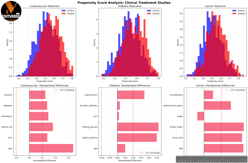
Propensity score distributions and standardized differences for cardiovascular, diabetes, and cancer treatment studies. The overlap between treated and control groups indicates the quality of matching potential.
Covariate Balance Assessment in Clinical Research
Before and after matching, we assess covariate balance using standardized differences, a critical component of propensity matching. Research published in Journal of Medical Internet Research emphasizes the importance of balance assessment for study validity.
Balance Assessment Criteria
- Standardized differences < 0.1 (excellent balance)
- Standardized differences < 0.2 (adequate balance)
- Statistical significance testing (p > 0.05 after matching)
- Visual assessment of propensity score overlap
Propensity Matching Algorithm for Clinical Research
The core of propensity matching involves implementing robust matching algorithms. Furthermore, we use 1:1 nearest neighbor matching with caliper restrictions to ensure high-quality matches, as recommended by The BMJ.
Treatment Effect Estimation in Clinical Research
After successful matching, we estimate treatment effects using various statistical methods. Additionally, we calculate risk differences, odds ratios, and hazard ratios depending on the outcome type, as outlined in JAMA guidelines.

Treatment effect estimates and balance assessment after propensity matching for cardiovascular readmission, diabetes HbA1c reduction, and cancer survival outcomes.
Sensitivity Analysis for Clinical Research
Robust propensity matching requires comprehensive sensitivity analysis. Moreover, we test the stability of our results across different caliper values and matching methods, as recommended by Circulation.

Sensitivity analysis showing treatment effect stability across different caliper values and propensity score overlap assessment.
Sensitivity Analysis Components
- Varying caliper values (0.1, 0.2, 0.3)
- Different matching algorithms (nearest neighbor, optimal)
- Subgroup analyses by patient characteristics
- Assessment of unmeasured confounding
Clinical Applications of Propensity Matching
Propensity matching has numerous applications in modern medicine. Specifically, it’s widely used in cardiovascular research, oncology, and pharmacoepidemiology, as documented in The New England Journal of Medicine.
Treatment effectiveness studies, device comparisons, medication safety
Survival analysis, treatment sequencing, biomarker studies
Drug safety, comparative effectiveness, real-world evidence
Conclusion and Best Practices for Clinical Research
Congratulations! You’ve mastered the fundamentals of propensity matching. Here’s what you’ve learned from our introduction, clinical datasets, and comprehensive analysis:
Key Takeaways
- Propensity score calculation using logistic regression
- Covariate balance assessment with standardized differences
- 1:1 nearest neighbor matching with caliper restrictions
- Treatment effect estimation and interpretation
- Comprehensive sensitivity analysis
- Real-world clinical applications
Remember that successful propensity matching requires careful attention to balance assessment, transparent reporting, and thorough sensitivity analysis. Furthermore, always consider the clinical relevance of your findings and their implications for patient care.
Ready to Apply Propensity Matching Clinical Research?
Download the complete Python code and datasets to start your own propensity matching projects. Additionally, explore our other tutorials on Q-Q plots for clinical data analysis and advanced statistical methods.
Download Complete Code